- The document discusses signals and systems problems and solutions. - It provides examples of signals, systems, and their properties including linearity, time-invariance, causality, stability, and invertibility. - It analyzes signals including impulse functions, step functions, and periodic functions. It also analyzes systems including integrators, differentiators, and cascaded systems.

1. 3 Signals and Systems: PartII
Solutions to
Recommended Problems
S3.1
(a)
x[n]= 8[n] + 8 [n - 3]
n
0 1 2 3
Figure S3.1-1
(b)
x[n] = u[n]-u[n-- 5]
1111
0041T
-1 0 1 2 3 4 5
Figure S3.1-2
(c)
x [n]=S[n] + -1 [n -- +(_1)2S[n] +(_1)3 5[n -3]
1 n
-3 -2 -1 0 1 2 3 4 5 6 7
Figure S3.1-3
(d)
x(t)= u(t +3) - u(t - 3)
t
-3 0 3
Figure S3.1-4
S3-1

2. Signals and Systems
S3-2
(e)
x(t) =6(t + 2)
-2 0
Figure S3.1-5
t
(f)
S3.2
(1)
(2)
(3)
(4)
(5)
(6)
h
d
b
e
a, f
None
S3.3
(a)
(b)
x[n] = b[n - 1] - 26[n - 2] + 36[n - 3]
s[n] = -u[n + 3] + 4u[n + 1] - 4u[n ­
- 26[n ­ 4]
2] + u[n -
+ b[n -
4]
5]
S3.4
We are given Figure S3.4-1.

3. Signals and Systems: Part II / Solutions
S3-3
x(- t) and x(1 - t) are as shown in Figures S3.4-2 and S3.4-3.
x (-t)
-12
Figure S3.4-2
x(1--t)
x1-0
(a)
-11 1
Figure S3.4-3
u(t + 1) - u(t - 2) is as shown in Figure S3.4-4.
Hence, x(1
-1
- t)[u(t + 1)
0 1 2
Figure S3.4-4
- u(t - 2)]1looks as in Figure S3.4-5.
t
-1
5
6
1
Figure S3.4-5
t

4. Signals and Systems
S3-4
(b) -u(2 - 3t) looks as in Figure S3.4-6.
2
3
t
Hence, u(t + 1)
Figure S3.4-6
- u(2 - 3t) is given as in Figure S3.4-7.
2
3
So x(1 ­ t)[u(t +
Figure S3.4-7
1) - u(2 - 3t)] is given as in Figure S3.4-8.
S3.5
(a) y[n]
(b) y[n]
(c) y[n]
(d) y[n]
=
=
=
=
x2[n] + x[n] -
x2[n] + x[n] -
H[x[n] ­ x[n -
x2[n] + x 2
[n -
G[x 2[n]]
x2
[n] - X2
[n -
x[n
x[n
1]]
1] -
1
- 1]
- 1]
2x[nJx[n ­ 1]

5. Signals and Systems: Part11/ Solutions
S3-5
(e) y[n] = F[x[n] - x[n - 1]]
= 2(x[n] - x[n - 1]) + (x[n - 1] - x[n - 2])
y[n] = 2x[n] - x[n - 1] - x[n - 2]
(f) y[n] = G[2x[n] + x[n - 11]
= 2x[n] + x[n - 11 - 2x[n - 1] - x[n - 21
= 2x[n] - x[n - 1] - x[n - 2]
(a) and (b) are equivalent. (e) and (f) are equivalent.
S3.6
Memoryless:
(a) y(t) = (2 + sin t)x(t) is memoryless because y(t) depends only on x(t) and not
on prior values of x(t).
(d) y[n] = Ek=. x[n] is not memoryless because y[n] does depend on values of
x[-] before the time instant n.
(f) y[n] = max{x[n], x[n - 1], ... , x[-oo]} is clearly not memoryless.
Linear:
(a) y(t) = (2 + sin t)x(t) = T[x(t),
T[ax1(t) + bx 2(t)] = (2 + sin t)[axi(t) + bx 2(tt)
= a(2 + sin t)x 1(t) + b(2 + sin t)x 2(t)
= aT[x1(t)] + bT[x 2(t)]
Therefore, y(t) = (2 + sin t)x(t) is linear.
(b) y(t) = x(2t) = T[x(t)],
T[ax1(t) + bx 2(t)] = ax1(2t) + bx 2(t)
= aT[x1 (t)) + bT[x 2(t)]
Therefore, y(t) = x(2t) is linear.
(c) y[n] = ( x[k] = T[x[n]],
k=­
T[ax1 [n] + bx2[n]] = a T x1[k] + b L x 2[k]
k= -x k=-w
= aT[x1[n]] + bT[x2[n]]
Therefore, yin] = E=_ x[k] is linear.
(d) y[n] = > x[k] is linear (see part c).
k= -o
dxt
d
T[ax1(t) + bx 2(t)] = -[ax 1 (t)+±bx
2(t)]
= a
dx
dt
1(t)
+ b
dx
dt
2(t)
= aT[x1(t)] + bT[x2(t)]
Therefore, y(t) = dx(t)/dt is linear.
(f) y[n] = max{x[n], . . . , x[-oo]} = T1x[n]],
T[ax1[n] + bx2[n]] = max{ax1[n] + bx 2[n], . . . , ax1[-oo] + bx2[ - o]}
# a max{x[n], . . . , x1[-oo]} + b max{x 2[n], . . . , X2[-00])
Therefore, y[n] = max{x[n], .. . , x[-oo]} is not linear.

6. Signals and Systems
S3-6
Time-invariant:
(a) y(t) = (2 + sin t)x(t) = T[x(t)],
T[x(t - T0 )] = (2 + sin t)x(t - T0 )
9 y(t - T0) = (2 + sin (t - T0))x(t - T0)
Therefore, y(t) = (2 + sin t)x(t) is not time-invariant.
(b) y(t) = x(2t) = T[x(t)],
T[x(t - T0 )] = x(2t - 2T0) # x(2t - TO) = y(t - T0 )
Therefore, y(t) = x(2t) is not time-invariant.
(c) y[n] = ( x[kJ = T[x[n]],
T[x[n - NO]J = ( x[k - NO] = y[n - N 0 ]
Therefore, y[n] = Ek'= _.x[k] is time-invariant.
(d) y[n] = E x[k] = T[x[n]],
k=­
n n-NO
T[x[n - NO]] = E x[k - N] = x[l] = y[n - N
0 ]
k=- =-w0
Therefore, y[n] = E" _.x[k] is time-invariant.
=dx(t)
(e) y(t) dt T[x(t)],
d
T[x(t - To)] = x(t - To) = y(t - To)
dt
Therefore, y(t) = dx(t)/dt is time-invariant.
Causal:
(b) y(t) = x(2t),
y(1) = x(2)
The value of y(-) at time = 1 depends on x(-) at a future time = 2. Therefore,
y(t) = x(2t) is not causal.
(d) y[n] = ( x[k]
k=­
Yes, y[n] = E .x[k] is causal because the value of y[-] at any instant n
depends only on the previous (past) values of x[-].
Invertible:
(b) y(t) = x(2t) is invertible; x(t) = y(t/2).
(c) y[n] = E _.x[k] is not invertible. Summation is not generally an invertible
operation.
(e) y(t) = dx(t)/dt is invertible to within a constant.
Stable:
(a) If Ix(t) I < M, Iy(t) I < (2 + sin t)M.Therefore, y(t) = (2 + sin t)x(t) is stable.
(b) If |x(t)| < M, |x(2t)I < M and ly(t)| < M. Therefore, y(t) = x(2t) is stable.
(d) If |x[k]| 5 M, ly[n]j 5 M - E_,, which is unbounded. Therefore, y[n] =
E"Lx[k] is not stable.

7. Signals and Systems: Part II / Solutions
S3-7
S3.7
(a) Since H is an integrator, H-1 must be a differentiator.
H~': y(t)
dx(t)
= d
dt
G: y(t) = x(2t)
G 1: y(t) = x(t/2)
(b)
Solutions to
Optional Problems
S3.8
(a) x 2(t) = xi(t) - xi(t - 2)
2(t) = 1(t) y)(t - 2)
Figure S3.8-1

8. Signals and Systems
S3-8
(b) xA(t) = Xi( t) + xI(t + 1)
y3(t)=y (t)+y 1 (t + 1)
(c) x(t) = u(t - 1)
-1
- u(t - 2)
10 1 2
Figure S3.8-2
y(t)=e-(t-1)u
-1)+u(-t)+
u(t
-
2)
-u(1
-
t)
t
(d) y[n] = 3y 1[n] ­
p
2y2[n] +
2
p14
Figure S3.8-3
2y3[n]
3 3
p n
-3 -2 -1 0 1 2 3
-4
Figure S3.8-4

9. Signals and Systems: Part11/ Solutions
S3-9
(e) y2[n] = y,[n] + yi[n - 11
y2 [n] 2 __
0 1 2 3 4 5
Figure S3.8-5
Y3[n] = y 1 [n + 1]
-1 0 2 3 4
Figure S3.8-6
(f) From linearity,
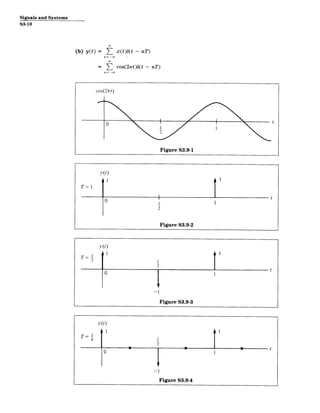
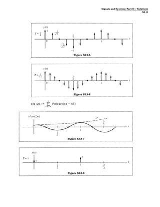
y1(t) = 1r + 6 cos(2t) - 47 cos(5t) + '/e cos(6t),
1 + 0t 4"
x 2(t) = 1 + t2 = (-t 2
)".
n=O
So y 2(t) = 1 - cos(2t) + cos(4t) - cos(6t) + cos(8t).
S3.9
(a) (i) The system is linear because
Tlaxi(t) + bx 2(t)] = 3 [ax1(t) + bx 2(t)](t - nT)
n=­
= a T3 x1 (t)b(t - nT) + b ( xst - nT)
= aT[xi(t)] + bT[x 2(t)]
(ii) The system is not time-invariant. For example, let xi(t) = sin(22rt/T).
The corresponding output yi(t) = 0. Now let us shift the input xi(t) by
r/2 to get
+r =
cos (2)
x 2 (t) = sin (
Now the output
+00
Y2(0 >7 b(t - nT) =Ay, + 2= 0
n = -oo

10. Signals and Systems
S3-10
(b) y(t) = E x(t)b(t - nT)
= E cos(2,rt)b(t - nT)
cos(27rt)
0< t
Figure S3.9-1
T = 1
0
I ~11 tt
2
Figure S3.9-2

11. Signals and Systems: Part II / Solutions
S3-11
y (t)
T=
T~__ t t
-1
Figure S3.9-5
y(t)
(c) y(t) = et
cos(27rt)b(t
Figure S3.9-6
- nT)
etcos(2nrt)
22
Figure S3.9-7
et
t
T = I
y (t)
T=1 tt
1
Figure S3.9-8
3
2

12. Signals and Systems
S3-12
y (t)
T= Ie3
2 2
-e1/2
I
I
2
2-
I 3/2
t
Figure S3.9-9
T=
4t
y (t)
YWe3
F r2
-el2
2
-e 3 12
Figure S3.9-10
T= Y3
12
1 y~t)
1
2
2
Figure S3.9-12
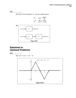
S3.10
(a) True. To see that the system is linear, write
y2 (t) = T2 [T1 [x(t)]] T[x(t)],
T1[ax1(t) + bx 2(t)] = aT1 [x1(t)] + bT[x2(t)]
T2[T1[ax1(t) + bx 2 (t)]] = T2[aT1[x1(t)] + bT1[x 2(t)]I
= aT2[T1[x1(t)]] + bT2[(T[x2t)]]
= aT[x1(t)] + bT[x 2(t)J

13. Signals and Systems: Part 11/ Solutions
S3-13
We see that the system is time-invariant from
T2[T1
[x(t - T)]] = T2[y1(t - T)l
= y 2(t -T),
Tx(t - T)] = y 2(t - T)
(b) False. Two nonlinear systems in cascade can be linear, as shown in Figure S3.10.
The overall system is identity, which is a linear system.
x(t) i Reciprocal -
1
x(t)
Reciprocal 0 y(t)=x(t)
Figure S3.10
(c) y[n] = z[2n] = w[2n] + {w[2n - 1] + {w[2n - 21
= x[n] + {x[n - 11
The system is linear and time-invariant.
(d) y[n] = z[-nl = aw[-n ­ 11 + bw[-n] + cw[-n + 1]
= ax[n + 11 + bx[nl + cx[n - 1]
(i) The overall system is linear and time-invariant for any choice of a, b,
and c.
(ii) a= c
(iii) a= 0
S3.11
(a) y[n] = x[n] + x[n - 11 = T[x[n]]. The system is linear because
T[ax1[n] + bx2[n]| = ax1[n] + ax1[n - 1] + bx 2[n] + bx2[n - 1]
= aT[x1 [n]] + bT[x 2[n - 1]]
The system is time-invariant because
y[n] = x[n] + x[n - 1] = Tjx[n]],
T[x[n - N]] = x[n - N] + x[n ­ 1 - N]
= y[n - N]
(b) The system is linear, shown by similar steps to those in part (a). It is not
time-invariant because
T[x[n ­ N]] = x[n - N]
# y[n - N]
+ x[n - N - 1] + x[O]
= x[n ­ N] + x[n - N - 1] + x[-NJ
S3.12
(a) To show that causality implies the statement, suppose
x1(t) - yl(t) (input x1(t) results in output y1(t)),
x 2(t) - y2),
where y1(t) and y2(t) depend on x1(t) and x 2(t) for t < to. By linearity,
xI(t) - x 2(t) -+ y 1(t) - y 2(t)

14. Signals and Systems
S3-14
If Xi(t) = x 2(t) for t < to, then y1(t) = y2 (t) for t < to. Hence, if x(t) = 0 for
t < to, y(t) = 0 for t < to.
(b) y(t) = x(t)x(t + 1),
x(t) = 0 for t < to =* y(t) = 0, for t < to
This is a nonlinear, noncausal system.
(c) y(t) = x(t) + 1 is a nonlinear, causal system.
(d) We want to show the equivalence of the following two statements:
Statement 1 (S1): The system is invertible.
Statement 2 (S2): The only input that produces the output y[n] = 0 for all n is
x[n] = 0 for all n.
To show the equivalence, we will show that
S2 false S1 false and
S1 false S2 false
S2 false == S1 false: Let x[n] # 0 produce y[n] = 0. Then cx[n] == y[n] = 0.
S1 false S2 false: Let xi => yi and x 2 =* Y2. If x 1 # X2 but y1 = Y2, then
X1 - X2 0 0 but yi - yi = 0.
(e) y[n] = x 2
[n] is nonlinear and not invertible.

15. MIT OpenCourseWare
http://ocw.mit.edu
Resource: Signals and Systems
Professor Alan V. Oppenheim
The following may not correspond to a particular course on MIT OpenCourseWare, but has been
provided by the author as an individual learning resource.
For information about citing these materials or our Terms of Use, visit: http://ocw.mit.edu/terms.