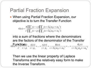
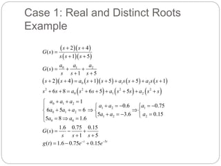
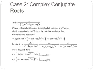
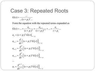
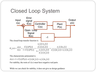
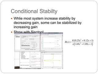
The document provides an outline for a lecture on loop transfer functions, Nyquist plots, and stability analysis. Key points include: - Partial fraction expansion can be used to analyze transfer functions with real distinct roots, complex conjugate roots, and repeated roots. - Open and closed loop transfer functions are defined. The characteristic polynomial determines stability for closed loop systems. 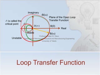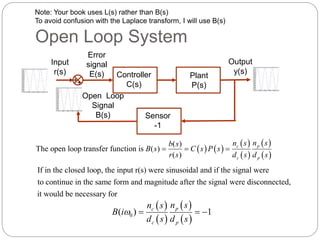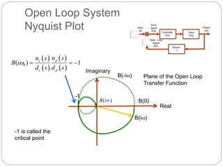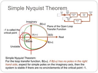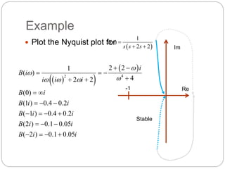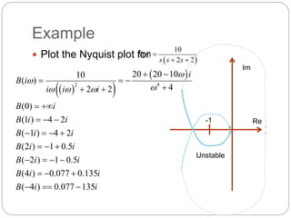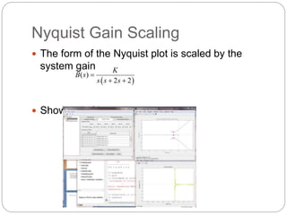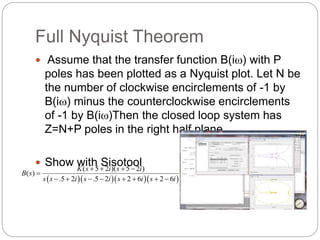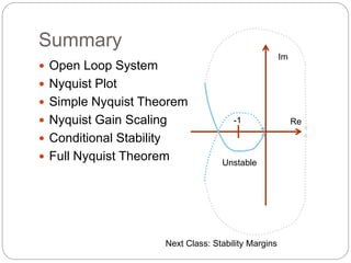- Nyquist plots involve evaluating the open loop transfer function B(s) as it traces a closed contour in the complex plane. The Nyquist stability criterion uses properties of this contour. - Heaviside expansion can be used to take the inverse Laplace transform of transfer functions with distinct poles.

1. Professor Walter W. Olson
Department of Mechanical, Industrial and Manufacturing Engineering
University of Toledo
Loop Transfer Function
-1
Real
Imaginary
Plane of the Open Loop
Transfer Function
B(0)
B(iw)
( )
B i
-1 is called the
critical point
Stable
Unstable
-B(iw)

2. Outline of Today’s Lecture
 Review
 Partial Fraction Expansion
 real distinct roots
 repeated roots
 complex conjugate roots
 Open Loop System
 Nyquist Plot
 Simple Nyquist Theorem
 Nyquist Gain Scaling
 Conditional Stability
 Full Nyquist Theorem

3. Partial Fraction Expansion
 When using Partial Fraction Expansion, our
objective is to turn the Transfer Function
into a sum of fractions where the denominators
are the factors of the denominator of the Transfer
Function:
Then we use the linear property of Laplace
Transforms and the relatively easy form to make
the Inverse Transform.
2
1 1
2
1 1
( ) ( 2 )
( )
( ) ( 2 )
m k
i i ni ni
i i
n q
r
i i ni ni
i i
K s z s s
G s
s s p s s
 w w
 w w
 
 
  

  
 
 
1 2 1
2 2
1 2 1 1 1
( )
( ) ( ) ( ) ( )
( ) ... ...
2 2
q
n
r
n n n q nq nq
B s
K A s A s A s B s
G s
s s p s p s p s s s s
 w w  w w
       
      

4. Case 1: Real and Distinct Roots
 
1
0 1 2
1 2
0 3 3
0
...
( )
( )
Put the transfer function in the form of
( ) ...
where the are called the residue at the pole
and determined by
( )
n
i
i
n
n
i i
s
G s
s s p
a a a a
G s
s s p s p s p
a p
a sG s a s p




    
  
  

 
       
3
1
2
1 1
2 2
( )
( ) ...
n
s p
s p
n n
s p s p
G s
a s p G s
a s p G s a s p G s


 
 
   

5. Case 1: Real and Distinct Roots
Example
  
  
         
     
0 1 2
0 1 2
2 2 2 2
0 1 2
0 1 2
1 2 1
0 1 2
1 2 2
0 0
2 4
( )
1 5
( )
1 5
2 4 1 5 5 1
6 8 6 5 5
1
0.6 0.75
6 5 6
5 3.6 0.15
5 8 1.6
1.6 0.75
( )
1
s s
G s
s s s
a a a
G s
s s s
s s a s s a s s a s s
s s a s s a s s a s s
a a a
a a a
a a a
a a a
a a
G s
s s
 

 
  
 
        
        
  

    
 

    
  
   
 
   

  

5
0.15
5
( ) 1.6 0.75 0.15
t t
s
g t e e
 

  

6. Case 2: Complex Conjugate
Roots
2 2
1
2
1 1 1
...
( )
... ( 2 )
We can either solve this using the method of matching coefficients
which is usually more difficult or by a method similar to that
previously used as follows:
2
q
i i i
i
G s
s s
s s
 w w
 w w


 
 

  
   
   
2
1 1 1 1
2
1 1 1 1
2 2
1 1 1 1 1 1 1 1
1 2
2 2 2 2
1 1 1 1 1 1 1 1
2
1 1 1 1 1 1
2
2 1 1 1 1 1
1 1
( )
then the term
2 1 1
proceeding as before
1
1
i i i
s
s
s s
A s a a
s s s s
a s G s
a s G s
 w w 
 w w 
 w w   w w 
 w w  w w   w w 
 w w 
 w w 
  
  
      
 
       
   
   

7. Case 3: Repeated Roots
 
 
1 1
1
1
2
2 2
3
3
...
( )
...( ) ...
Form the equation with the repeated terms expanded as
( ) ... ... ...
( ) ( )
( ) ( )
( )
( )
i
n
i
n n
n n
i i i
n
n i s p
n
n i
s p
n
n i
s p
n
G s
s p
a a a
G s
s p s p s p
a s p G s
d
a s p G s
ds
d
a s p G s
ds
d
a
ds










    
  
 
 
 
 
 
 
 
  
 
3
1
1 1
( )
...
( )
n
i
s p
n
n
i
n s p
s p G s
d
a s p G s
ds


 
 

 
 
 
 

8. Heaviside Expansion
 
 
 
 
1
1
2
Heaviside Expansion Formula: L
where are the distinct roots of ( )
15( 2)
Example: ( )
( 2 25)
Roots of the denominator are 0, 1 4.899, and
i
n
b t
i
i
i
i
A s A b
e
d
B s B b
ds
b n B s
s
G s
s s s
i


 
   

   
 
   
 


 
 

 
 
 
   
   
2 2 2
3
1
2
1
1 4.899 1 4.899
0
1 4.899
15. 73.485i 15. 73.485i
48.0
1 4.899
( 2 25) 2 2 3 4 25
15( 2)
L
3 4 25
30
( )
25
(
0 9.798i 48.00 9.798i
0.6 1.408
) 1. i
2
i
i
s t
i s s
i t i t
t
i
i
d
B s s s s s s s
ds
s
G s e
s s
g t e e e
g t e

 
   
 
 
       

 
 
 


 
 
  
 
  
 

   
1 4.899
0.6 1.408i
t i t
e
 
 


9. Loop Nomenclature
Reference
Input
R(s)
+-
Output
y(s)
Error
signal
E(s)
Open Loop
Signal
B(s)
Plant
G(s)
Sensor
H(s)
Prefilter
F(s)
Controller
C(s)
+-
Disturbance/Noise
The plant is that which is to be controlled with transfer function G(s)
The prefilter and the controller define the control laws of the system.
The open loop signal is the signal that results from the actions of the
prefilter, the controller, the plant and the sensor and has the transfer function
F(s)C(s)G(s)H(s)
The closed loop signal is the output of the system and has the transfer function
( ) ( ) ( )
1 ( ) ( ) ( )
F s C s G s
C s G s H s


10. Closed Loop System
++
Output
y(s)
Error
signal
E(s)
Open Loop
Signal
B(s)
Plant
P(s)
Controller
C(s)
Input
r(s)
   
   
 
 
 
 
 
 
 
 
   
       
           
The closed loop transfer function is
( )
( )
( ) 1
1
The characteristic polynomial is
( ) 1
For stability, the roots of ( ) m
p
c
c p c p
yr
p
c c p c p
c p
c p c p
n s
n s
d s d s n s n s
C s P s
y s
G s
n s
n s
r s C s P s d s d s n s n s
d s d s
s C s P s d s d s n s n s
s


   
 

   
ust have negative real parts
While we can check for stability, it does not give us design guidance
-1

11. Open Loop System
++
Output
y(s)
Error
signal
E(s)
Open Loop
Signal
B(s)
Plant
P(s)
Controller
C(s)
Input
r(s)
   
 
 
 
 
( )
The open loop transfer function is ( )
( )
p
c
c p
n s
n s
b s
B s C s P s
r s d s d s
  
Note: Your book uses L(s) rather than B(s)
To avoid confusion with the Laplace transform, I will use B(s)
Sensor
-1
If in the closed loop, the input r(s) were sinusoidal and if the signal were
to continue in the same form and magnitude after the signal were disconnected,
it would be necessary for
 
 
 
 
0
( ) 1
p
c
c p
n s
n s
B i
d s d s
w   

12. Open Loop System
Nyquist Plot Error
signal
E(s)
++
Output
y(s)
Open Loop
Signal
B(s)
Plant
P(s)
Controller
C(s)
Input
r(s)
Sensor
-1
 
 
 
 
0
( ) 1
p
c
c p
n s
n s
B i
d s d s
w   
-1
Real
Imaginary
Plane of the Open Loop
Transfer Function
B(0)
B(iw)
( )
B i
-1 is called the
critical point
B(-iw)

13. Simple Nyquist TheoremError
signal
E(s)
++
Output
y(s)
Open Loop
Signal
B(s)
Plant
P(s)
Controller
C(s)
Input
r(s)
Sensor
-1
Simple Nyquist Theorem:
For the loop transfer function, B(iw), if B(iw) has no poles in the right
hand side, expect for simple poles on the imaginary axis, then the
system is stable if there are no encirclements of the critical point -1.
-1
Real
Imaginary
Plane of the Open Loop
Transfer Function
B(0)
B(iw)
( )
B i
-1 is called the
critical point
Stable
Unstable
-B(iw)

14. Example
 Plot the Nyquist plot for  
1
( )
2 2
B s
s s s

 
 
 
 
4
2
2 2
1
( )
4
2 2
(0)
(1 ) 0.4 0.2
( 1 ) 0.4 0.2
(2 ) 0.1 0.05
( 2 ) 0.1 0.05
i
B i
i i i
B i
B i i
B i i
B i i
B i i
w
w
w
w w w
 
  

 
 
  
   
  
   
-1
Im
Re
Stable

15. Example
 Plot the Nyquist plot for  
10
( )
2 2
B s
s s s

 
 
 
 
4
2
20 20 10
10
( )
4
2 2
(0)
(1 ) 4 2
( 1 ) 4 2
(2 ) 1 0.5
( 2 ) 1 0.5
(4 ) 0.077 0.135
( 4 ) 0.077 135
i
B i
i i i
B i
B i i
B i i
B i i
B i i
B i i
B i i
w
w
w
w w w
 
  

 
 
  
   
  
   
  
  
-1
Im
Re
Unstable

16. Nyquist Gain Scaling
 The form of the Nyquist plot is scaled by the
system gain
 Show with Sisotool
 
( )
2 2
K
B s
s s s

 

17. Conditional Stabilty
 Whlie most system increase stability by
decreasing gain, some can be stabilized by
increasing gain
 Show with Sisotool
 
2
2
(0.25 0.12 1)
( )
1.69 1.09 1
K s s
B s
s s s
 

 

18. Full Nyquist Theorem
 Assume that the transfer function B(iw) with P
poles has been plotted as a Nyquist plot. Let N be
the number of clockwise encirclements of -1 by
B(iw) minus the counterclockwise encirclements
of -1 by B(iw)Then the closed loop system has
Z=N+P poles in the right half plane.
 Show with Sisotool
    
( 5 2 )( 5 2 )
( )
.5 2 .5 2 2 6 2 6
K s i s i
B s
s s i s i s i s i
   

       

19. Summary
 Open Loop System
 Nyquist Plot
 Simple Nyquist Theorem
 Nyquist Gain Scaling
 Conditional Stability
 Full Nyquist Theorem
Next Class: Stability Margins
-1
Im
Re
Unstable