Download as PDF, PPTX


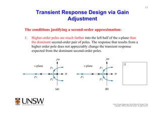


The document discusses root locus techniques, which provide a graphical representation of how the closed-loop poles of a system change with variations in system parameters like gain. It covers how to sketch root loci based on properties like starting/ending points and asymptotes. Design techniques are presented for using the root locus to meet transient response specifications by selecting gain values that place pole locations for good damping. Higher-order systems can be approximated as second-order to design gain for desired overshoot, settling time, etc.