Download as PDF, PPTX
![[course site]
Xavier Giro-i-Nieto
xavier.giro@upc.edu
Associate Professor
Universitat Politecnica de Catalunya
Technical University of Catalonia
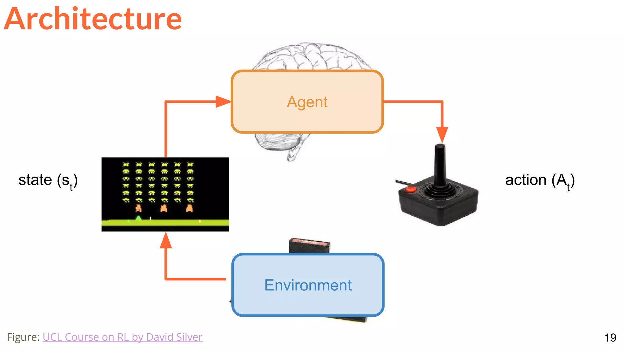
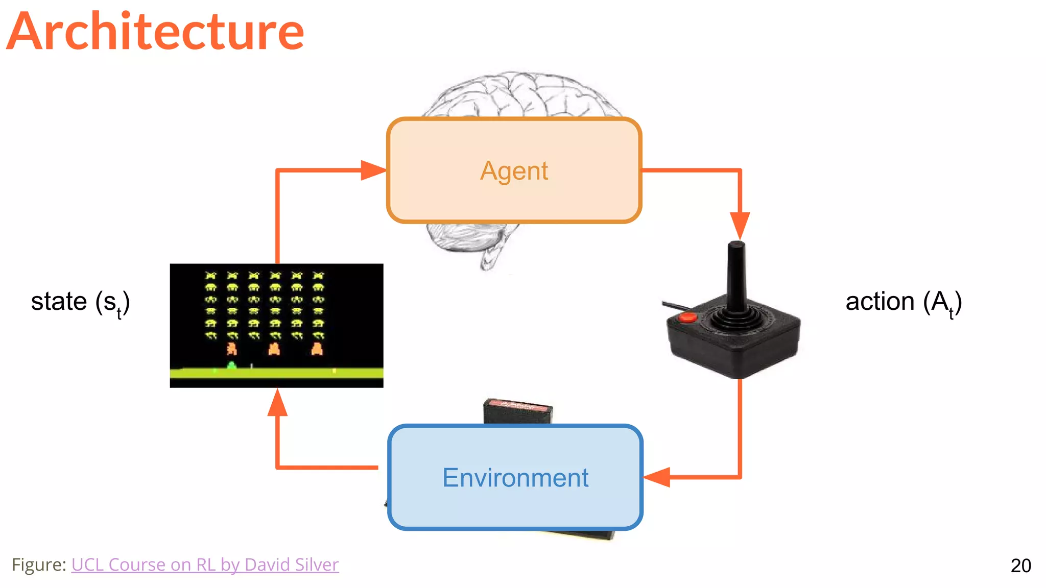
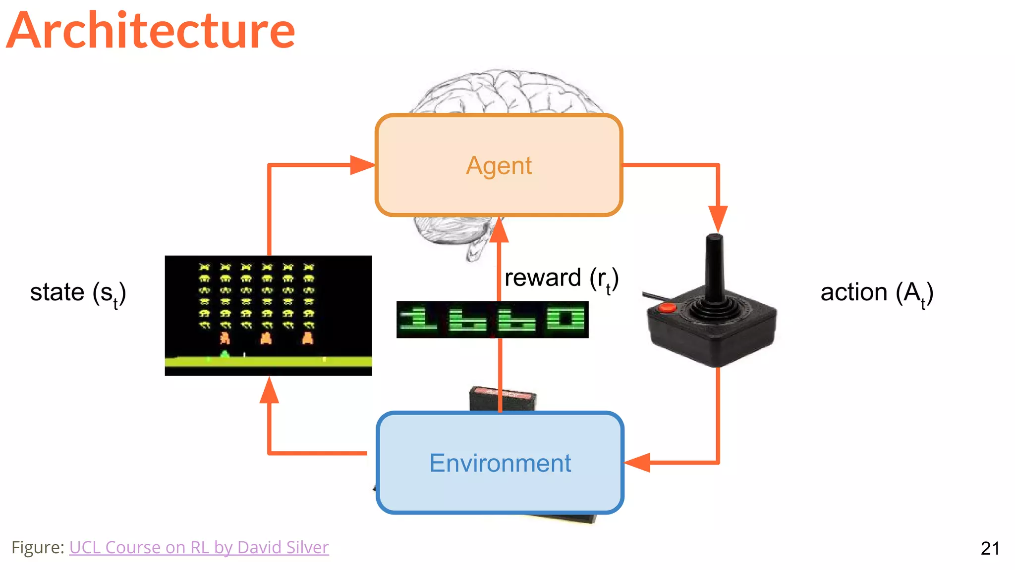
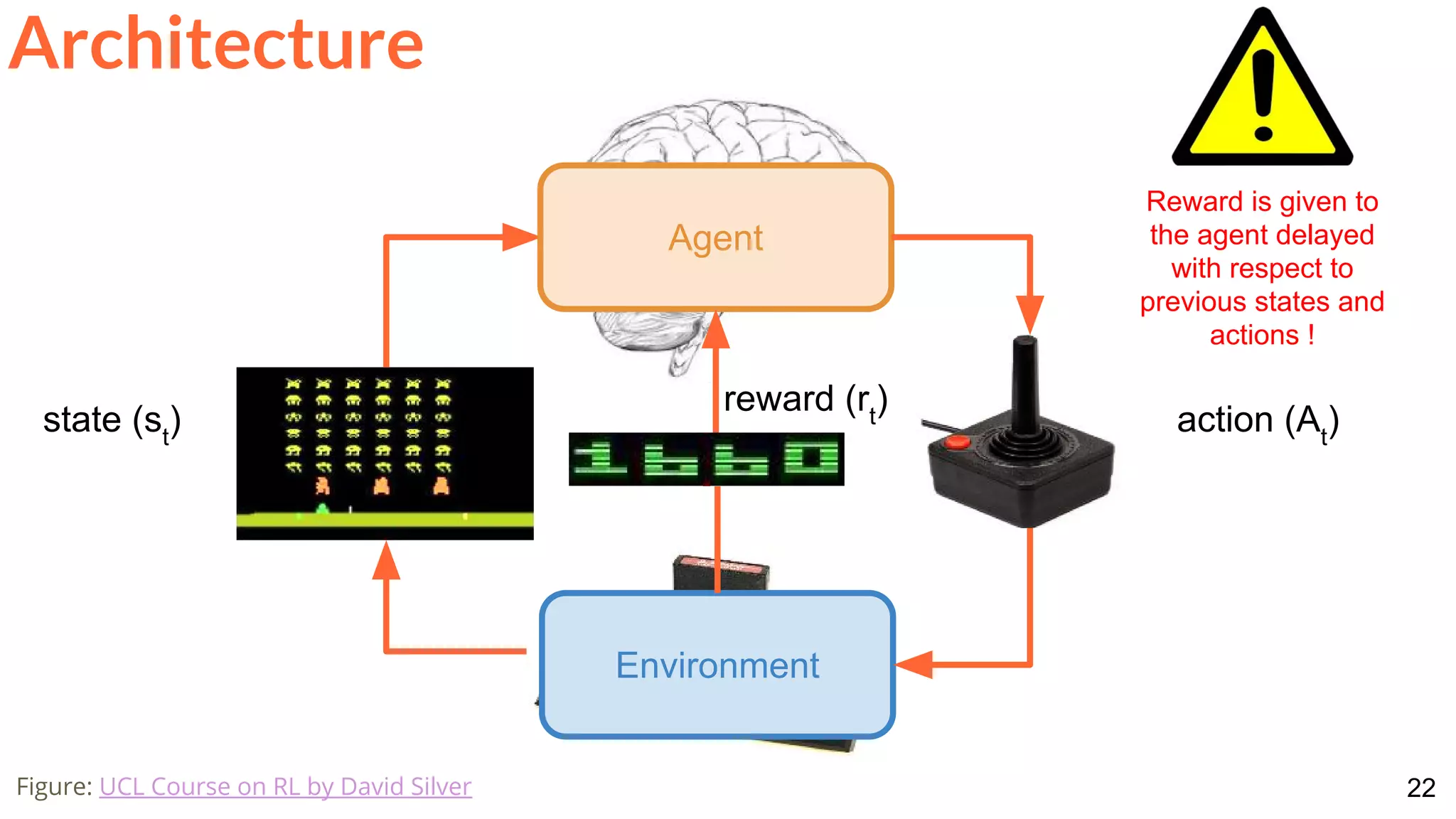
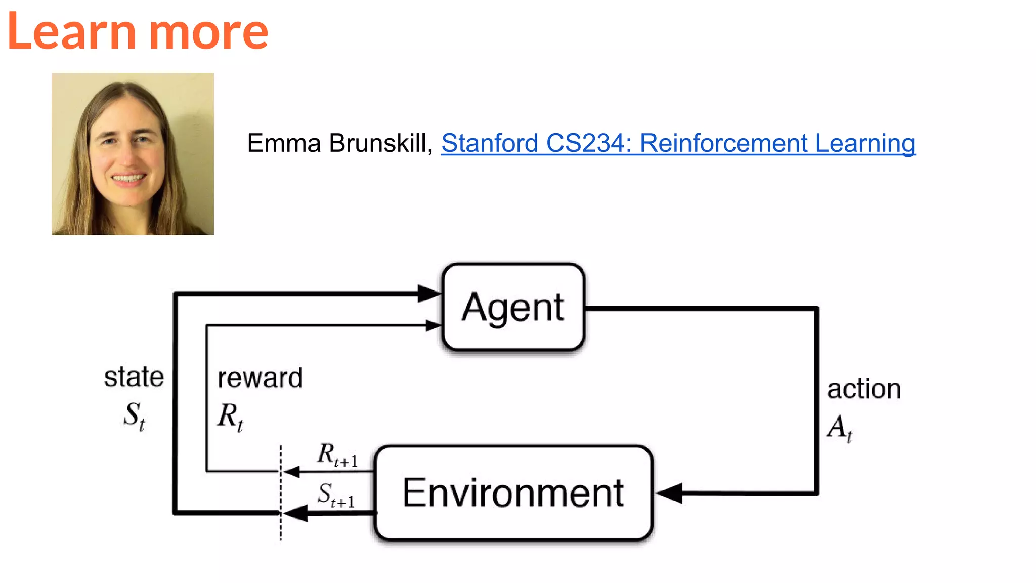
Reinforcement Learning
Day 7 Lecture 2
#DLUPC](https://image.slidesharecdn.com/dlai2017d7l2reinforcementlearning-171114180748/75/Reinforcement-Learning-DLAI-D7L2-2017-UPC-Deep-Learning-for-Artificial-Intelligence-1-2048.jpg)
![6
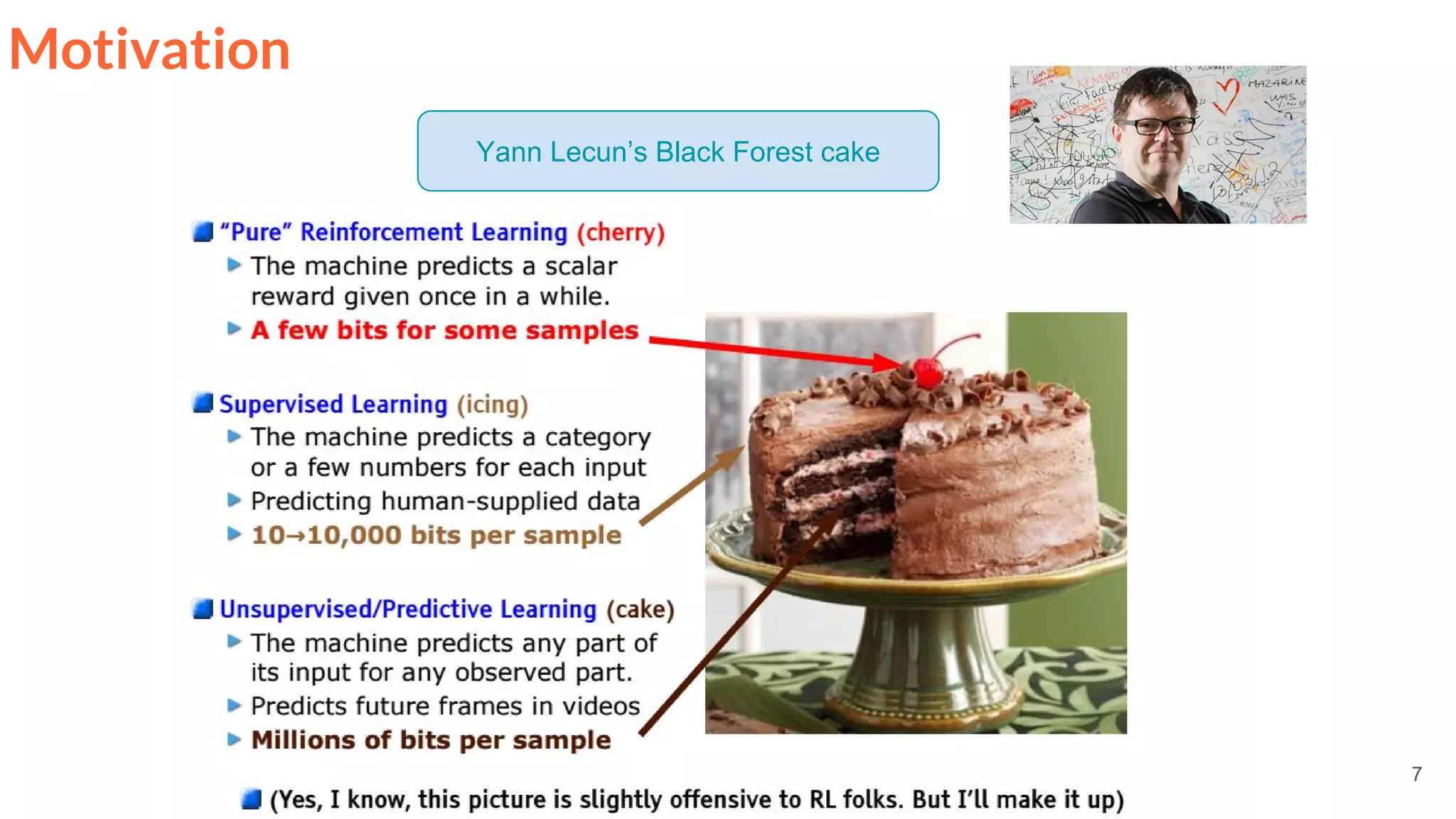
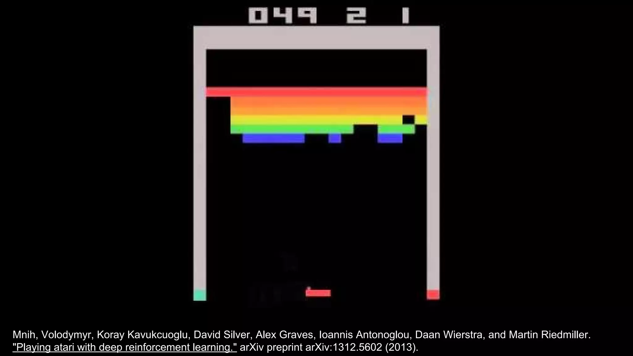
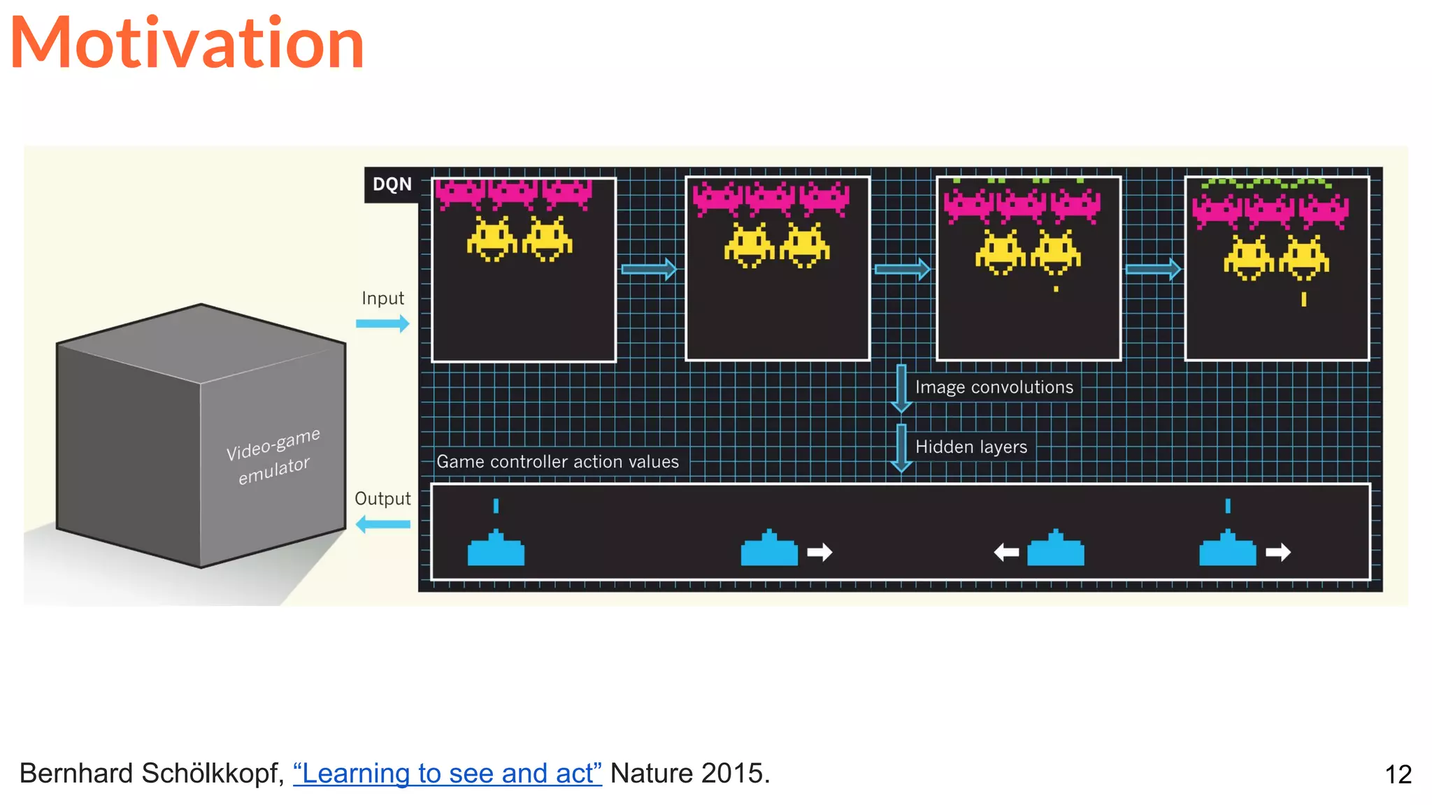
Motivation
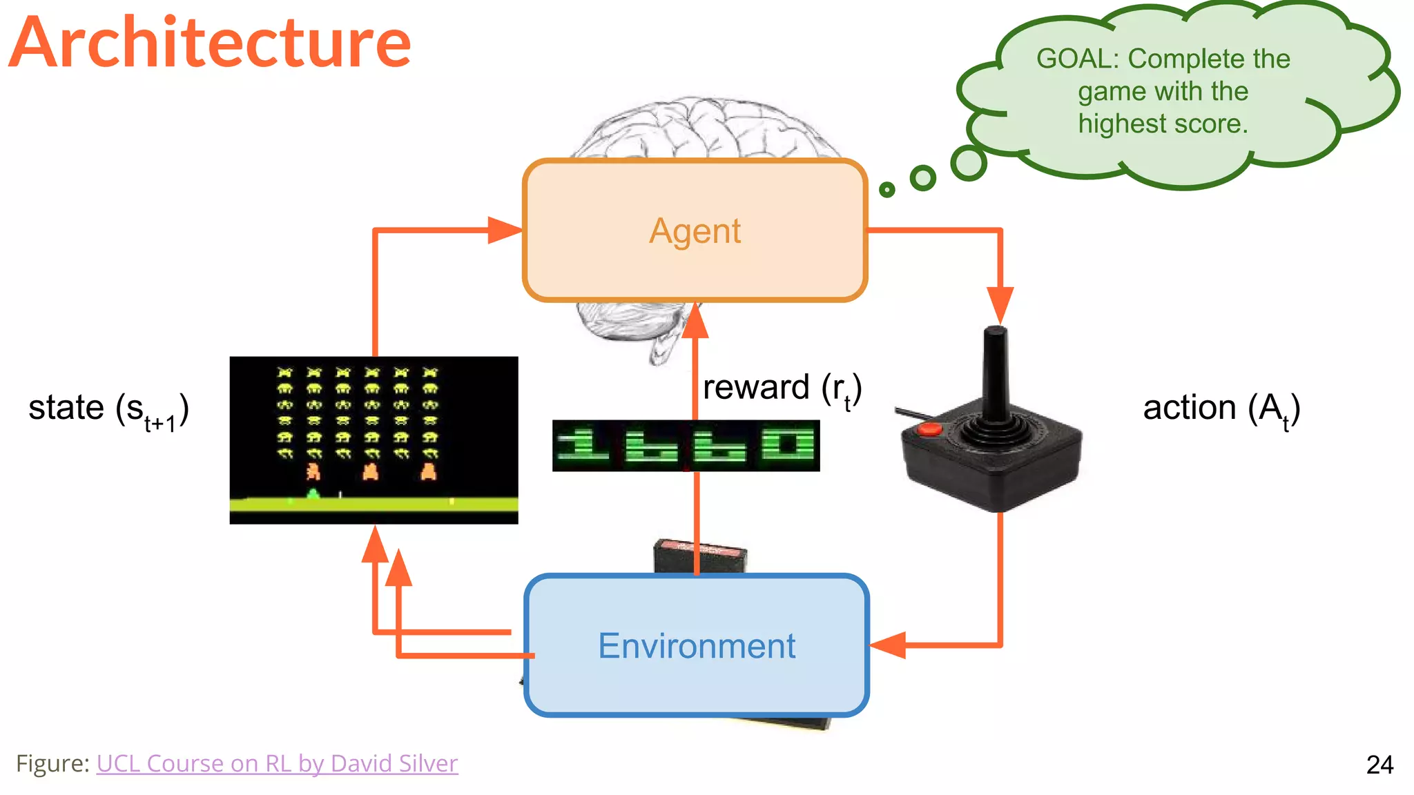
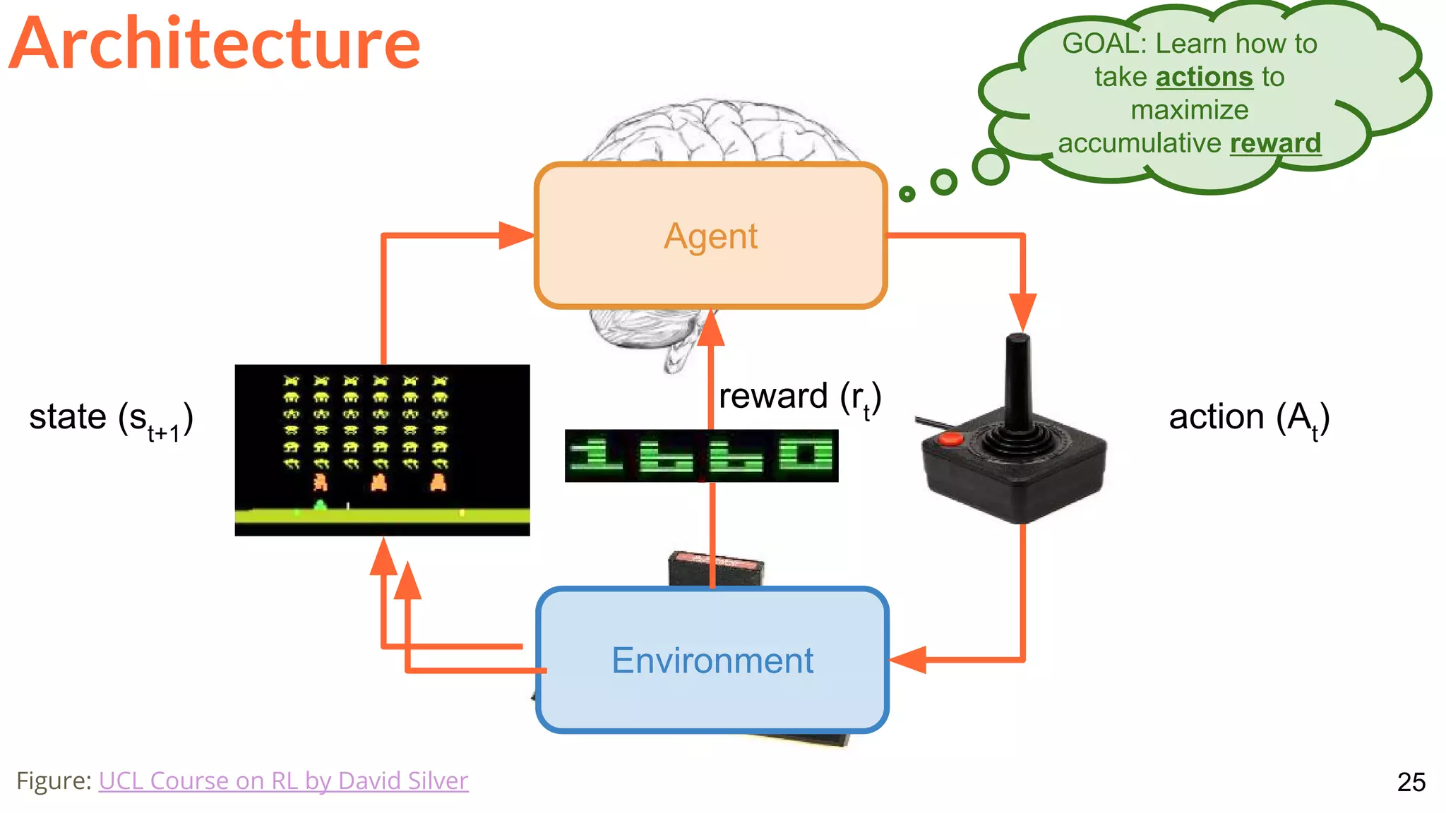
What is Reinforcement Learning ?
“a way of programming agents by reward and punishment without needing to
specify how the task is to be achieved”
[Kaelbling, Littman, & Moore, 96]
Kaelbling, Leslie Pack, Michael L. Littman, and Andrew W. Moore. "Reinforcement learning: A survey." Journal of artificial
intelligence research 4 (1996): 237-285.](https://image.slidesharecdn.com/dlai2017d7l2reinforcementlearning-171114180748/75/Reinforcement-Learning-DLAI-D7L2-2017-UPC-Deep-Learning-for-Artificial-Intelligence-6-2048.jpg)

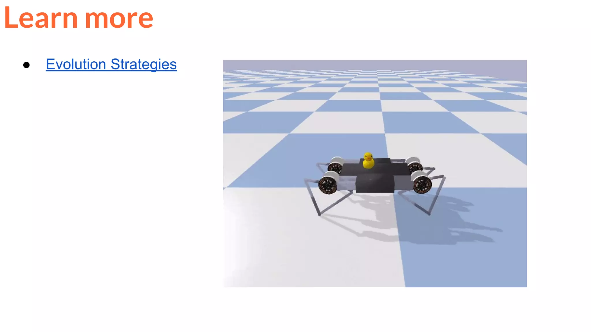
![28
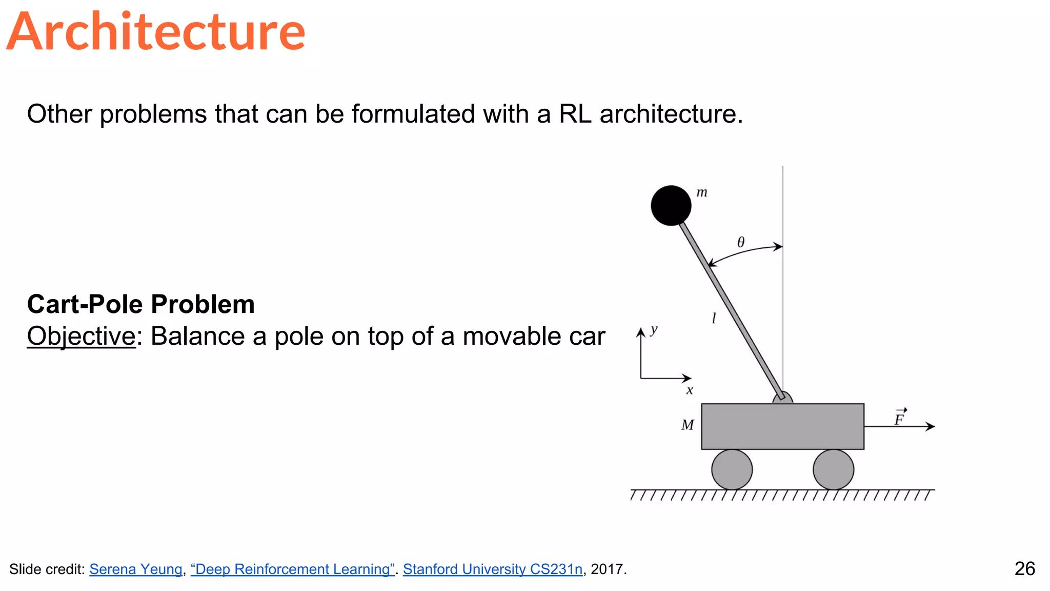
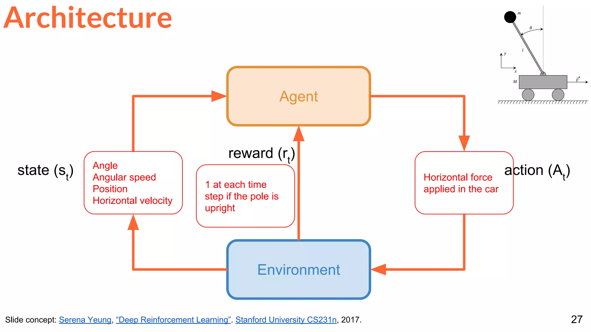
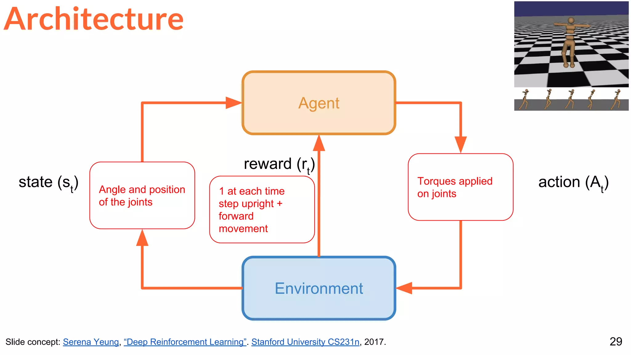
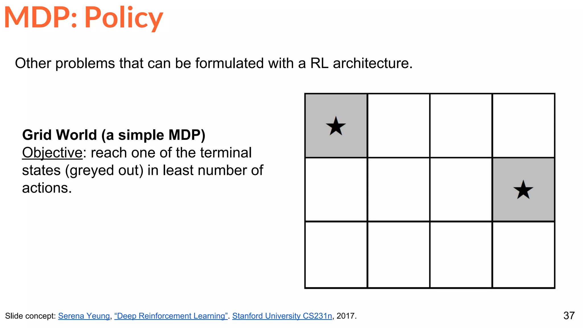
Other problems that can be formulated with a RL architecture.
Robot Locomotion
Objective: Make the robot move forward
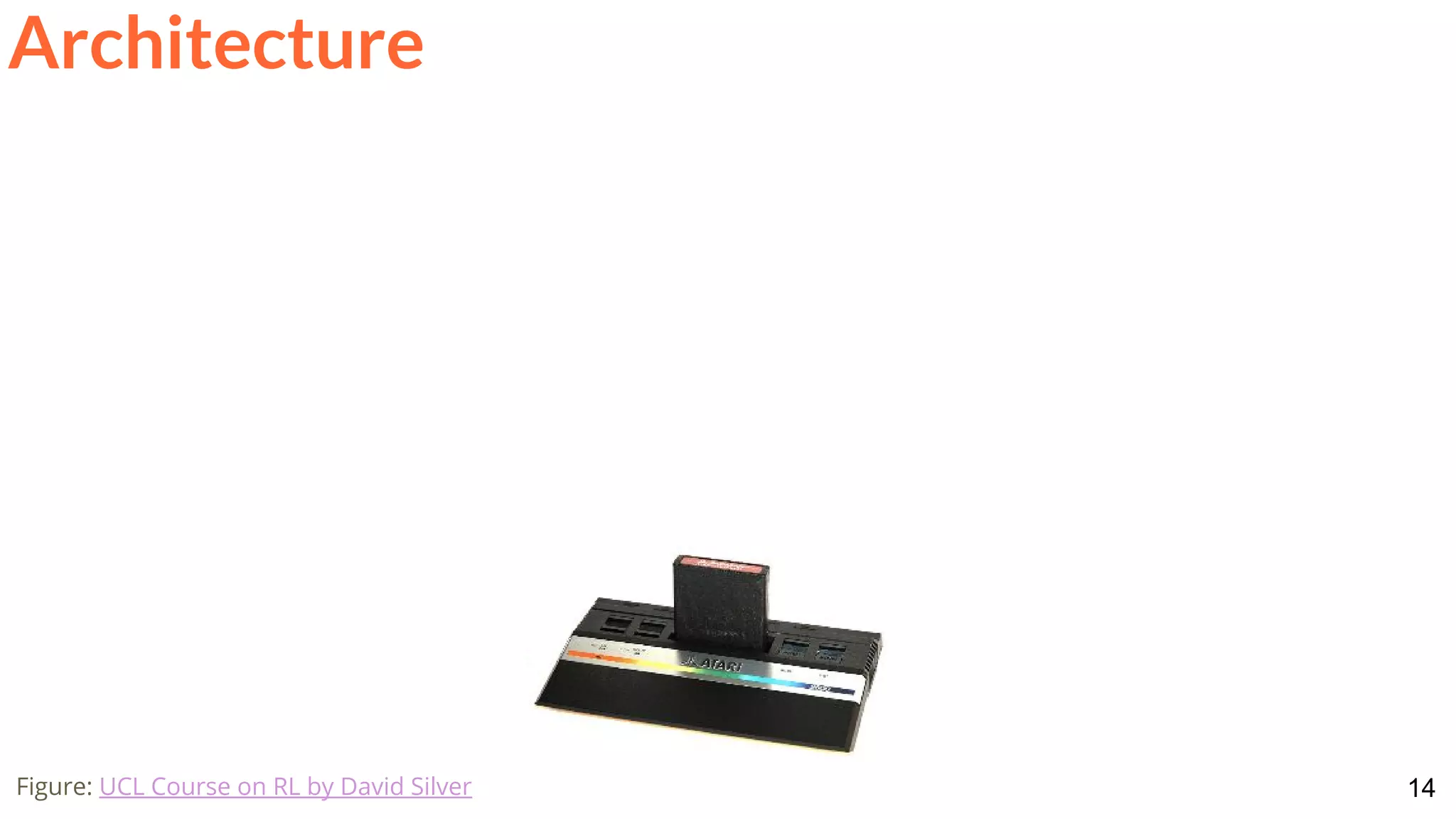
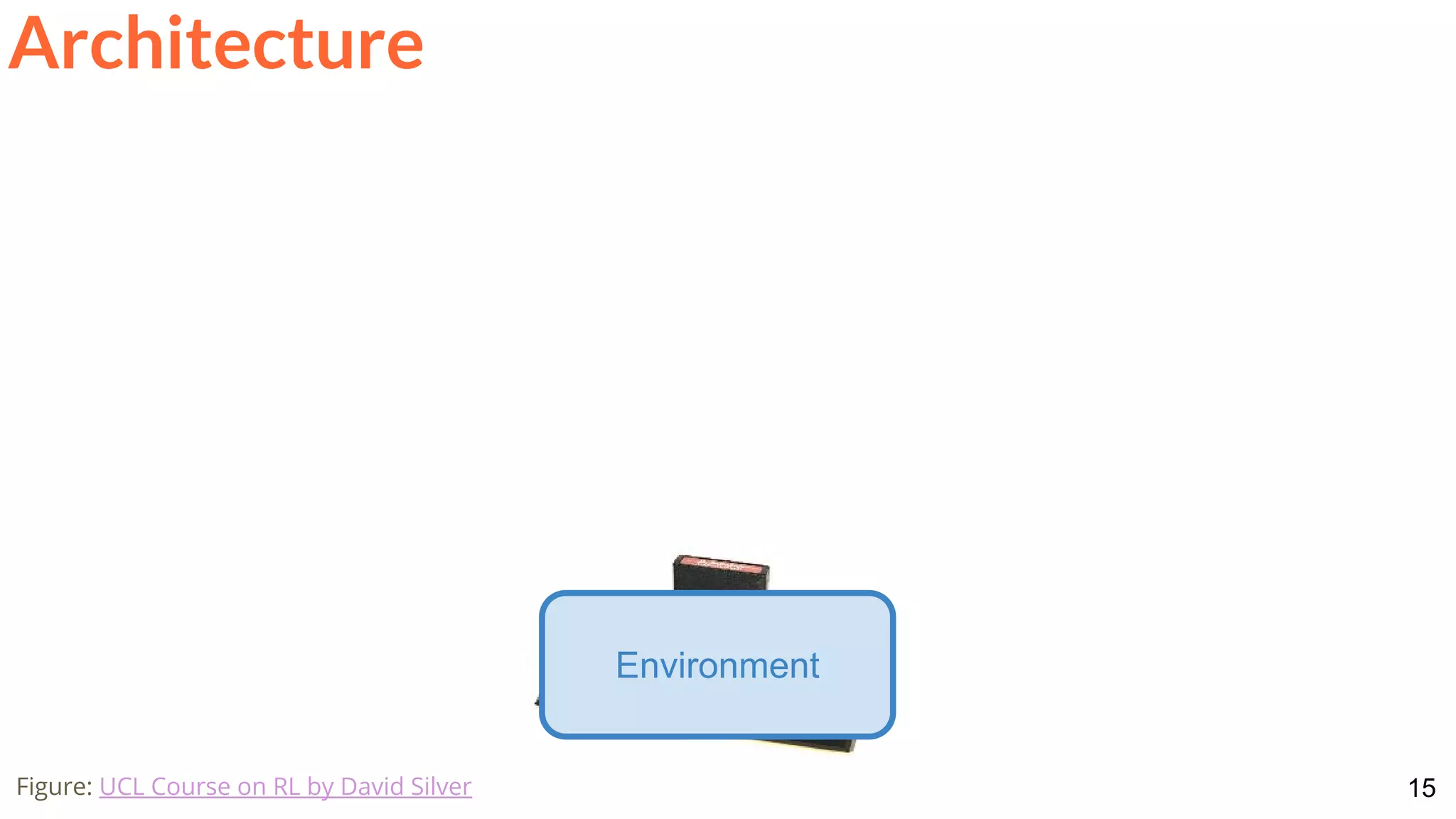
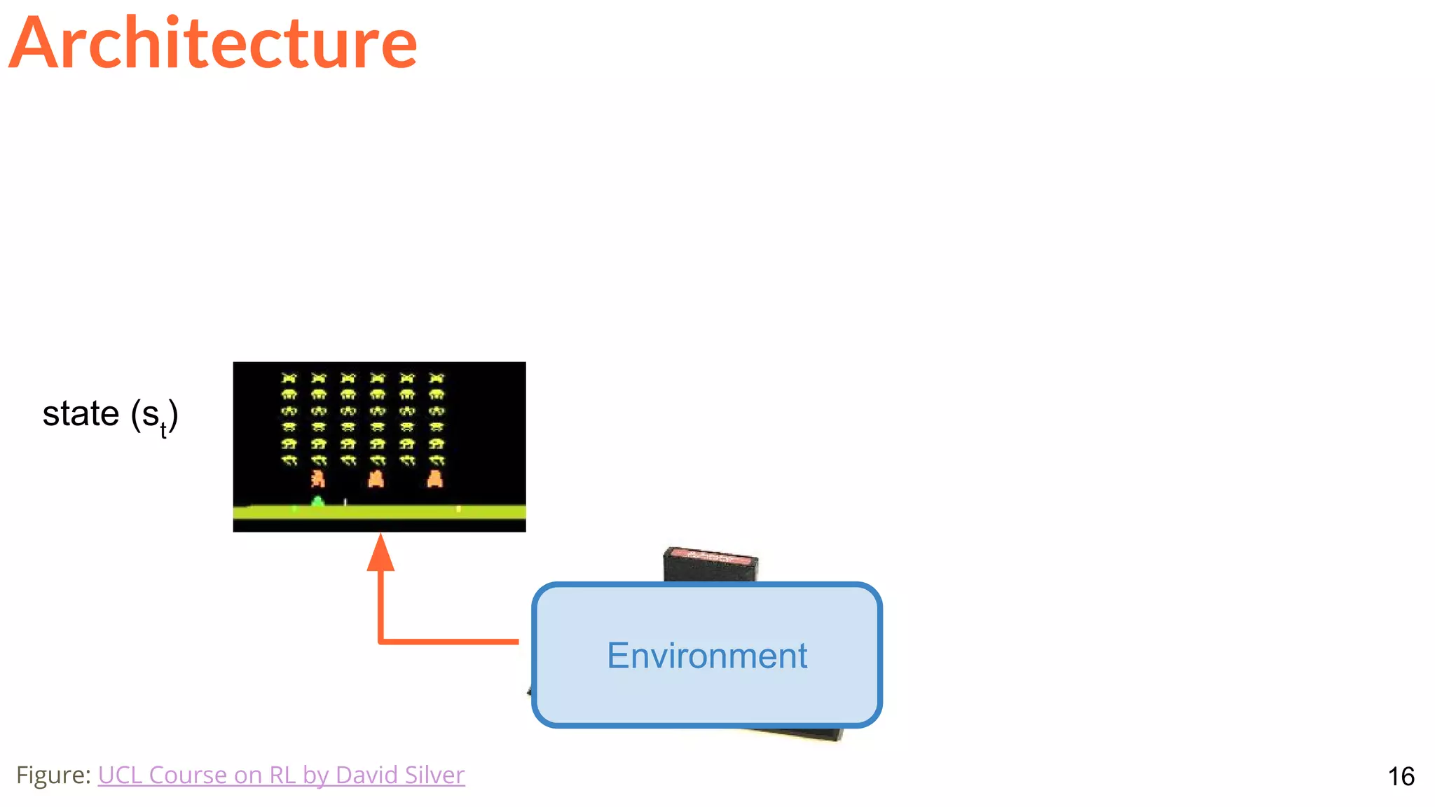
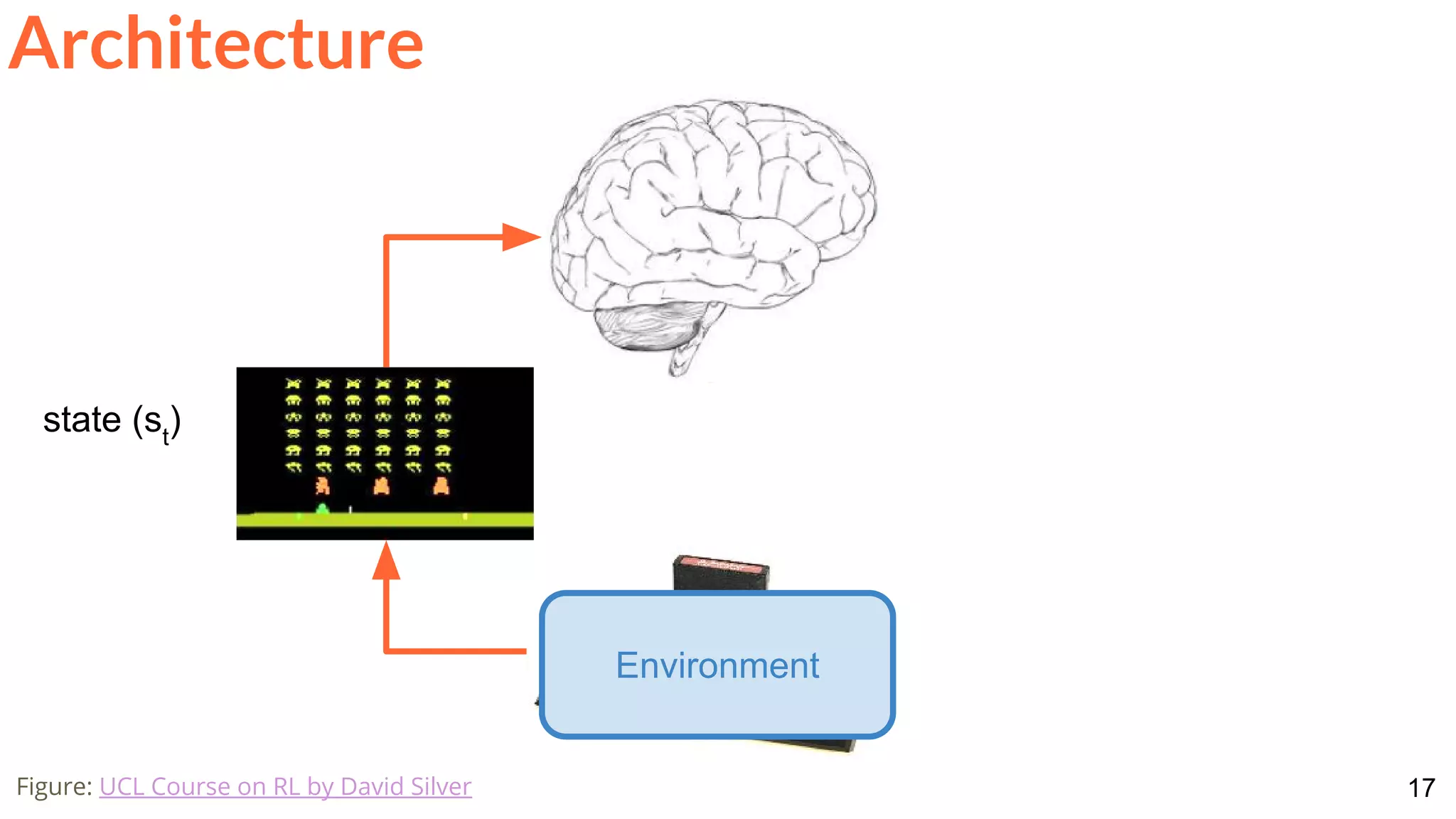
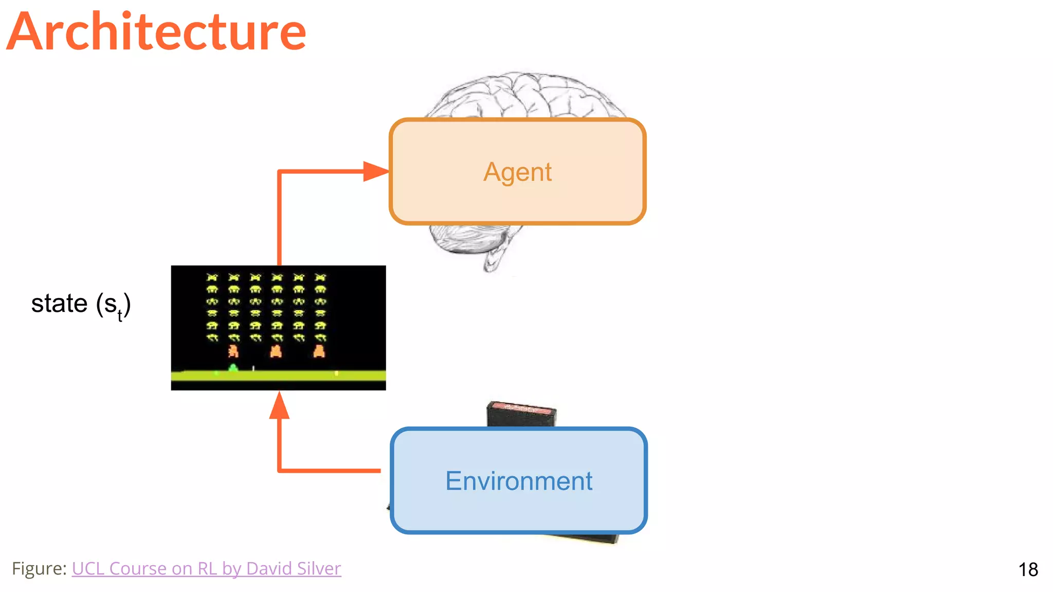
Architecture
Schulman, John, Philipp Moritz, Sergey Levine, Michael Jordan, and Pieter Abbeel. "High-dimensional continuous control using generalized
advantage estimation." ICLR 2016 [project page]](https://image.slidesharecdn.com/dlai2017d7l2reinforcementlearning-171114180748/75/Reinforcement-Learning-DLAI-D7L2-2017-UPC-Deep-Learning-for-Artificial-Intelligence-28-2048.jpg)
![30
Schulman, John, Philipp Moritz, Sergey Levine, Michael Jordan, and Pieter Abbeel. "High-dimensional continuous control using generalized
advantage estimation." ICLR 2016 [project page]](https://image.slidesharecdn.com/dlai2017d7l2reinforcementlearning-171114180748/75/Reinforcement-Learning-DLAI-D7L2-2017-UPC-Deep-Learning-for-Artificial-Intelligence-30-2048.jpg)

![86
Vinyals, O., Ewalds, T., Bartunov, S., Georgiev, P., Vezhnevets, A.S., Yeo, M., Makhzani, A., Küttler, H.,
Agapiou, J., Schrittwieser, J. and Quan, J., 2017. Starcraft ii: A new challenge for reinforcement learning.
arXiv preprint arXiv:1708.04782. [Press release]
Coming next...](https://image.slidesharecdn.com/dlai2017d7l2reinforcementlearning-171114180748/75/Reinforcement-Learning-DLAI-D7L2-2017-UPC-Deep-Learning-for-Artificial-Intelligence-86-2048.jpg)
![87
Vinyals, O., Ewalds, T., Bartunov, S., Georgiev, P., Vezhnevets, A.S., Yeo, M., Makhzani, A., Küttler, H.,
Agapiou, J., Schrittwieser, J. and Quan, J., 2017. Starcraft ii: A new challenge for reinforcement learning.
arXiv preprint arXiv:1708.04782. [Press release]
Coming next...](https://image.slidesharecdn.com/dlai2017d7l2reinforcementlearning-171114180748/75/Reinforcement-Learning-DLAI-D7L2-2017-UPC-Deep-Learning-for-Artificial-Intelligence-87-2048.jpg)

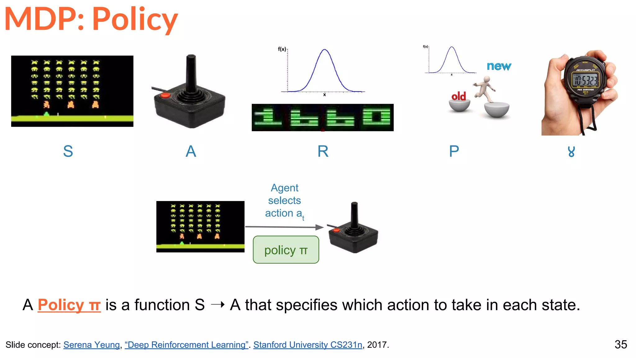
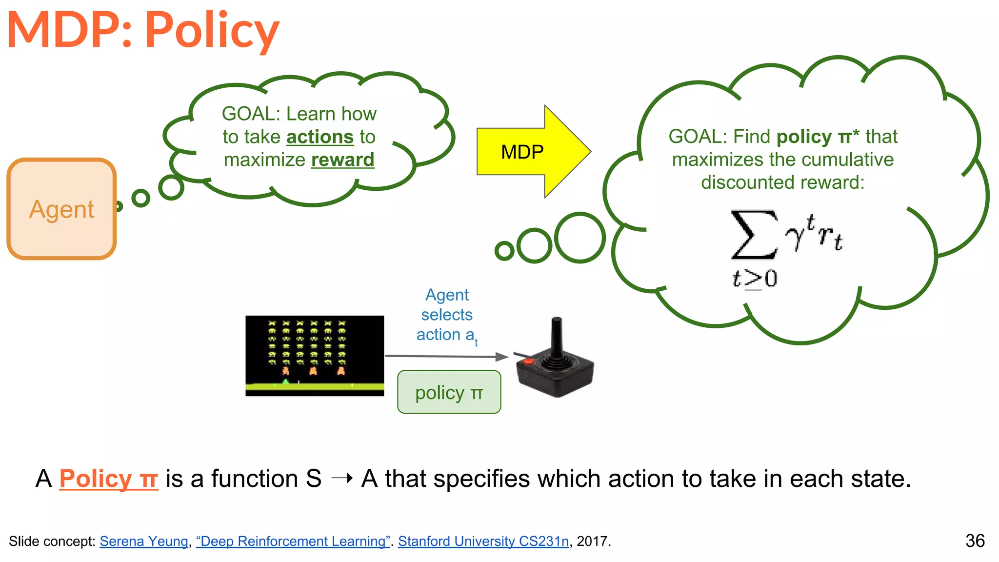
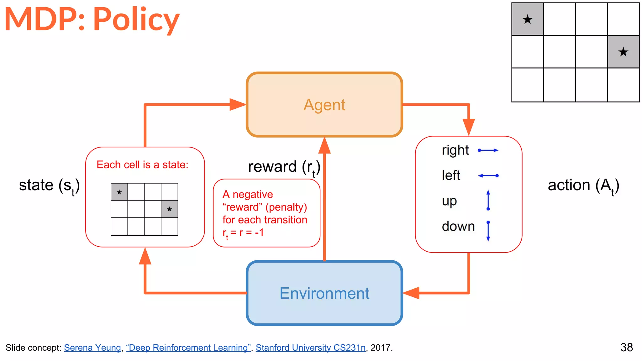
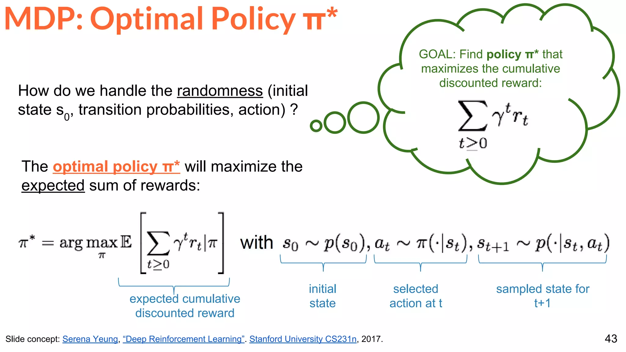
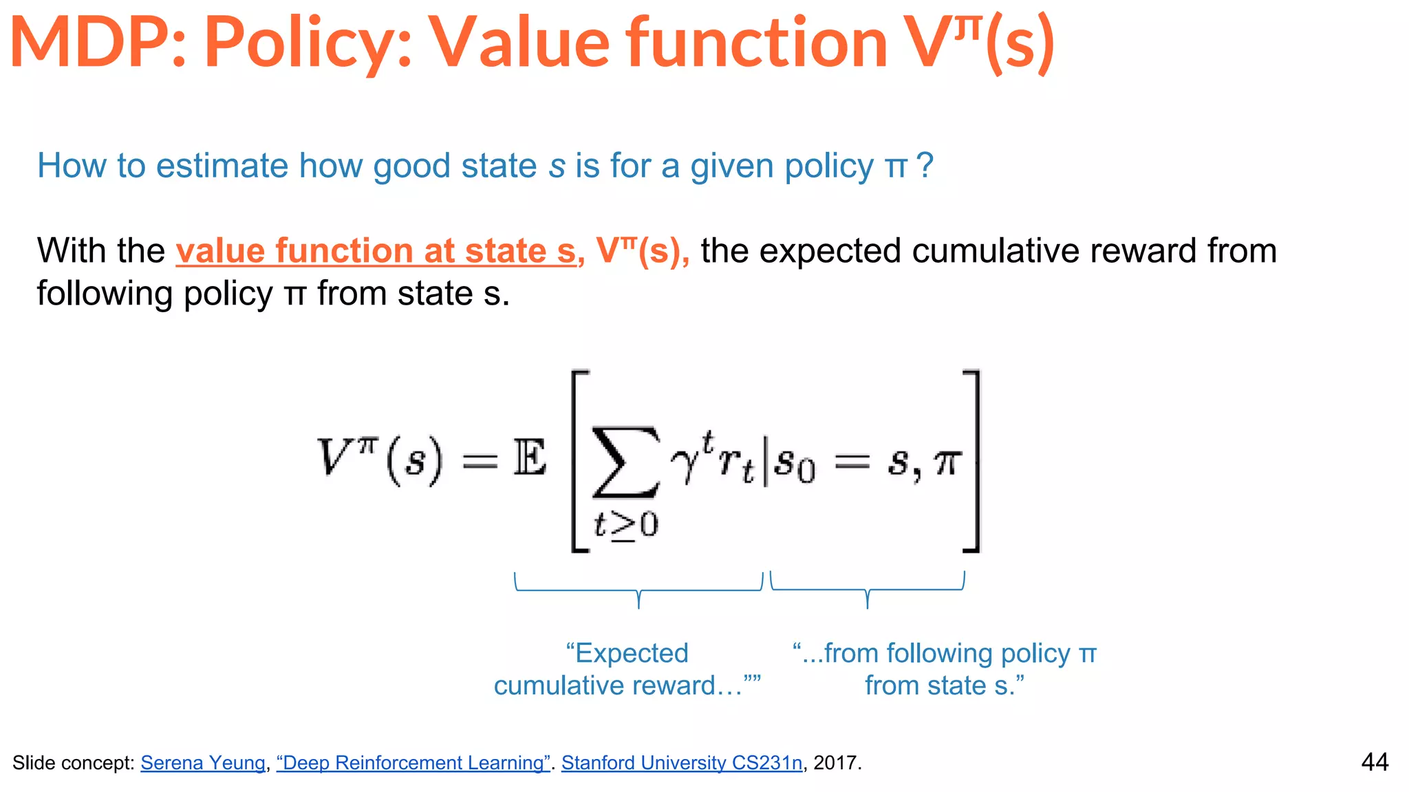
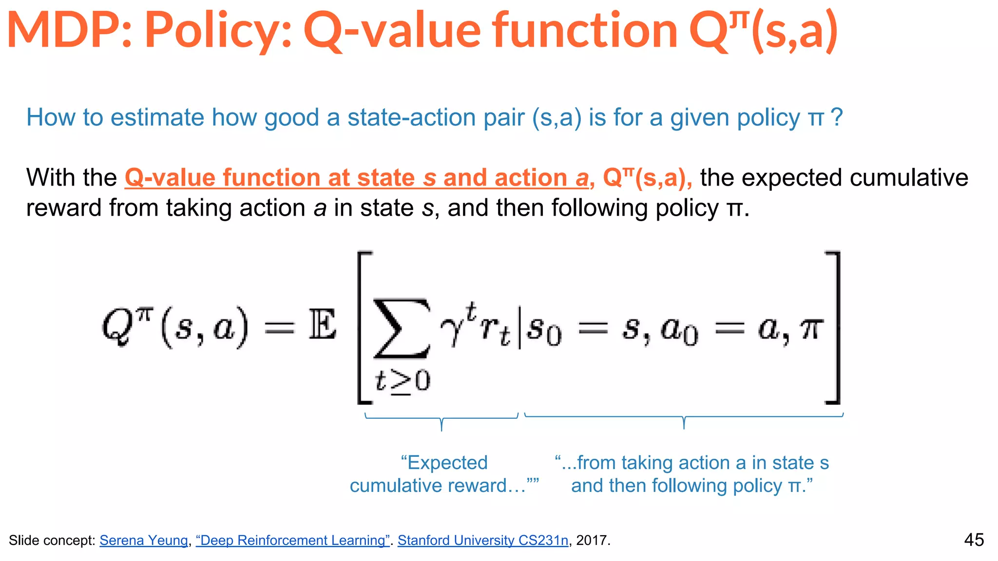
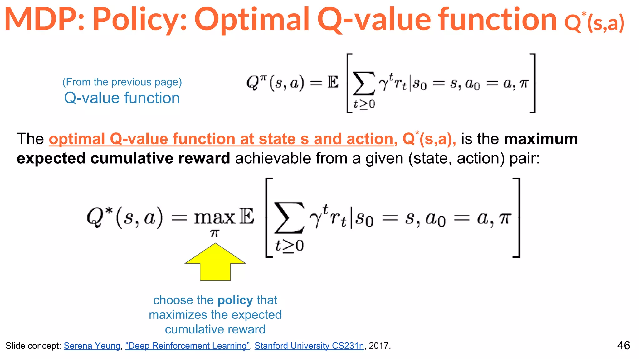
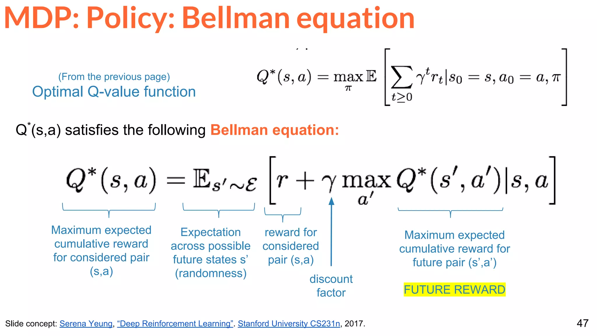
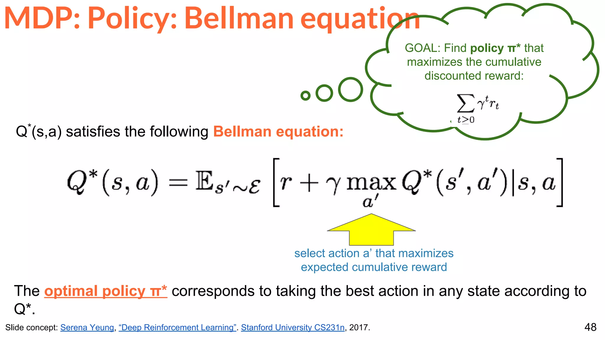
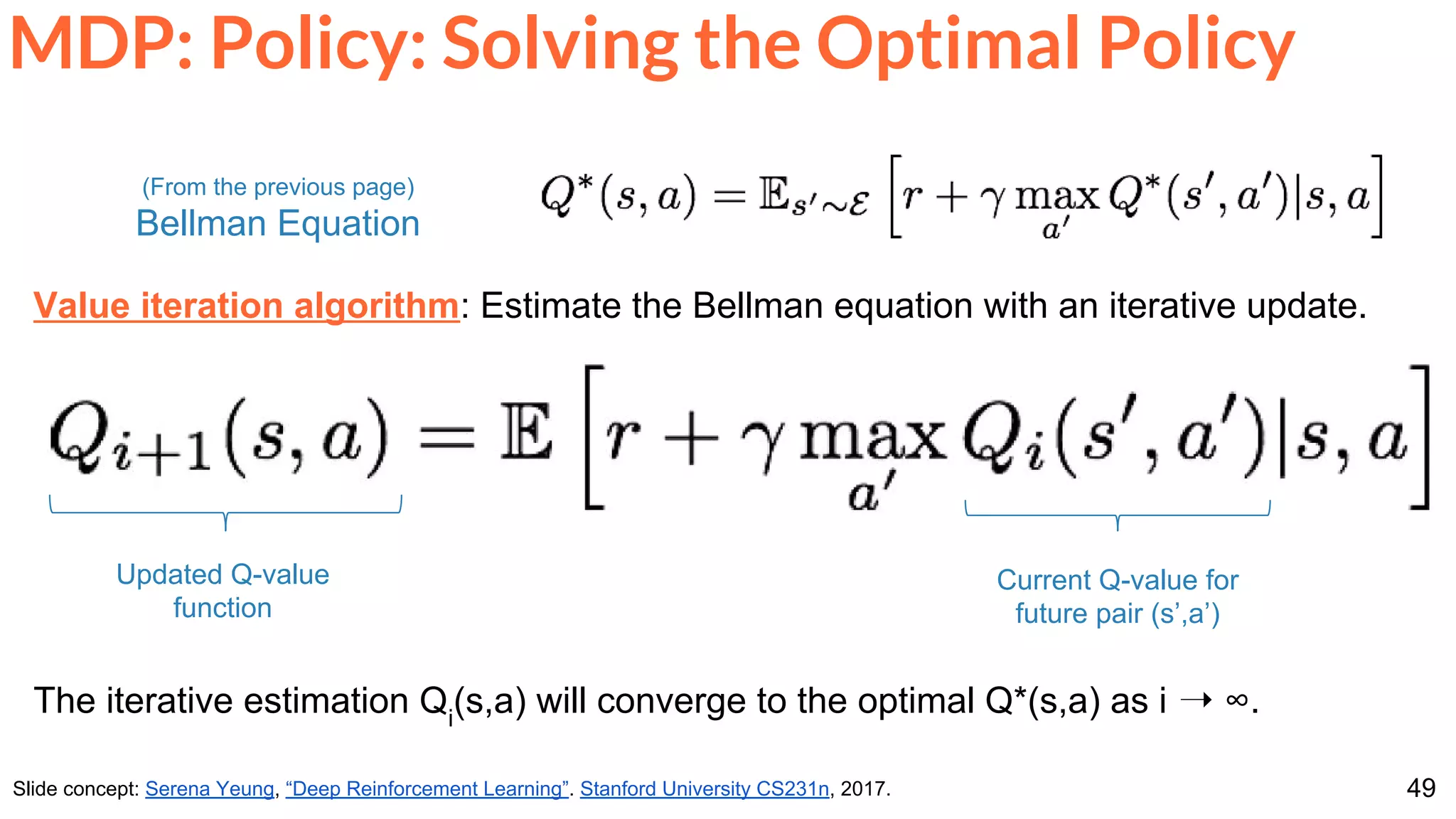
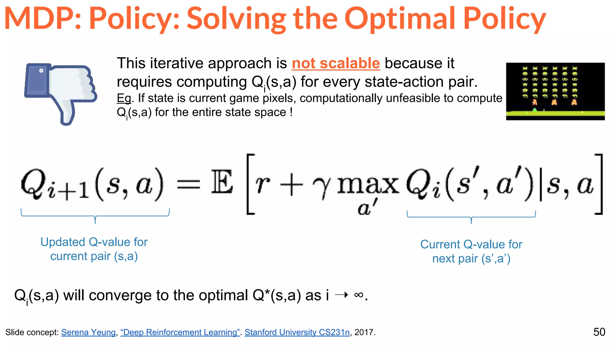
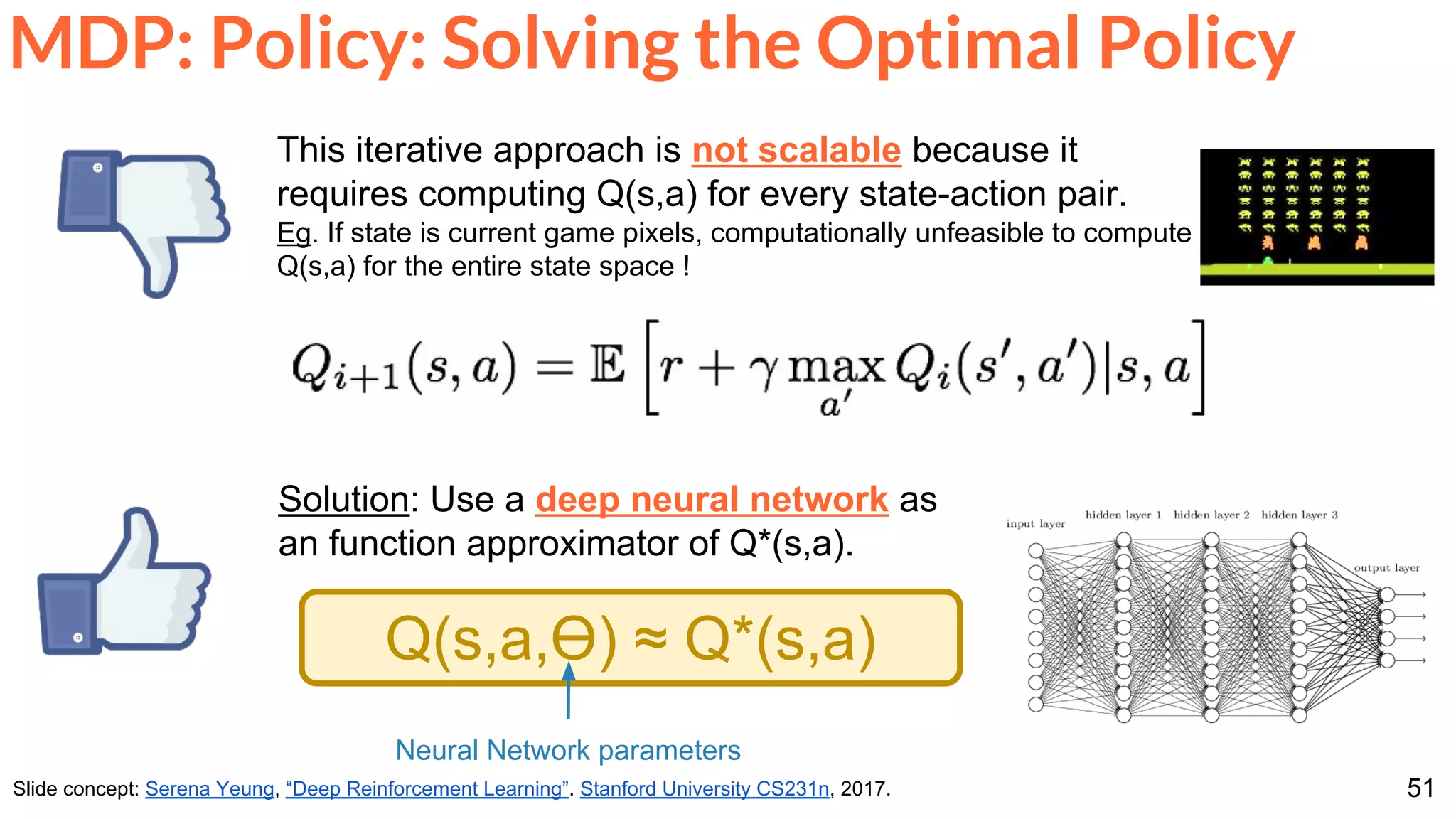
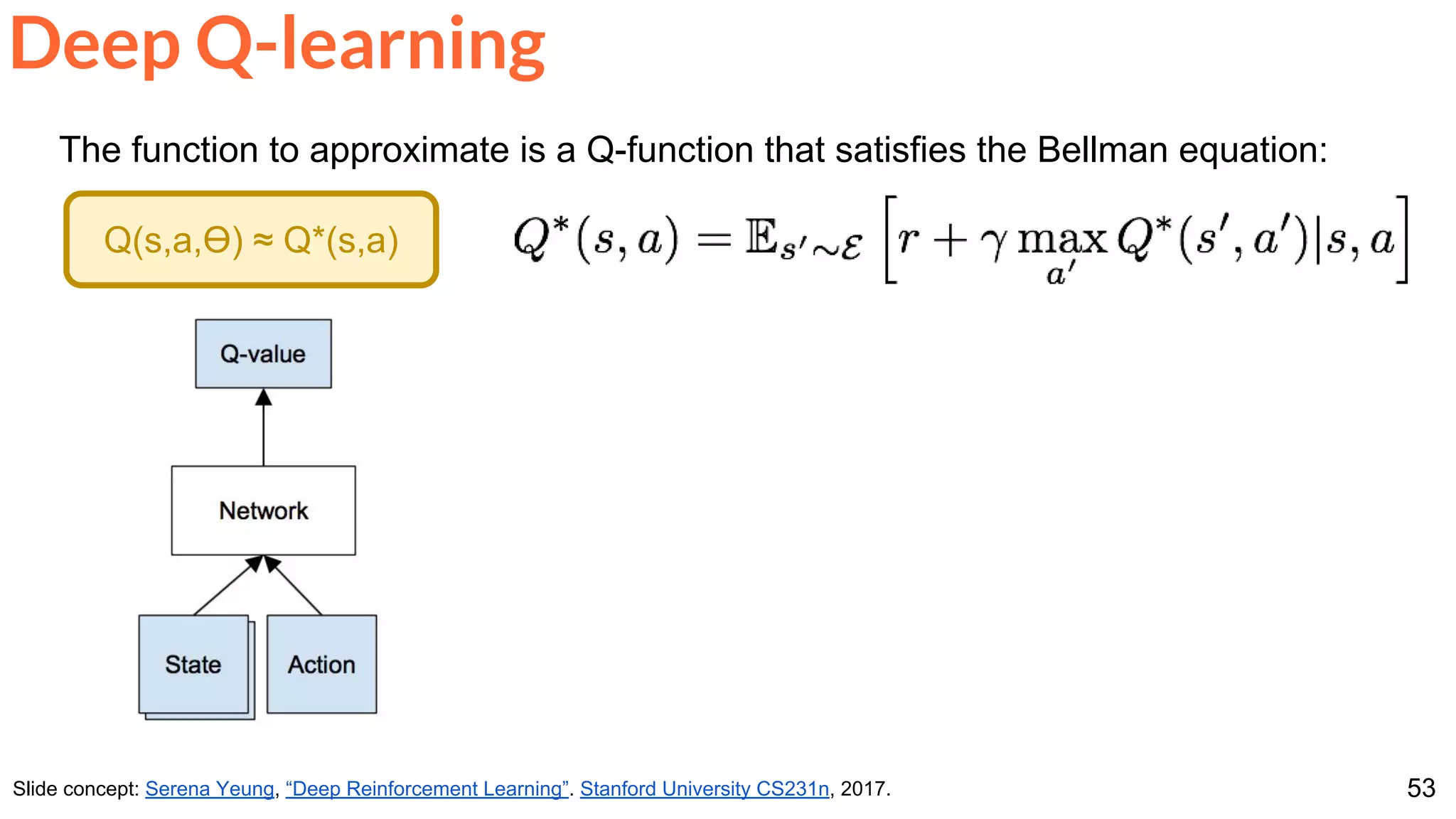
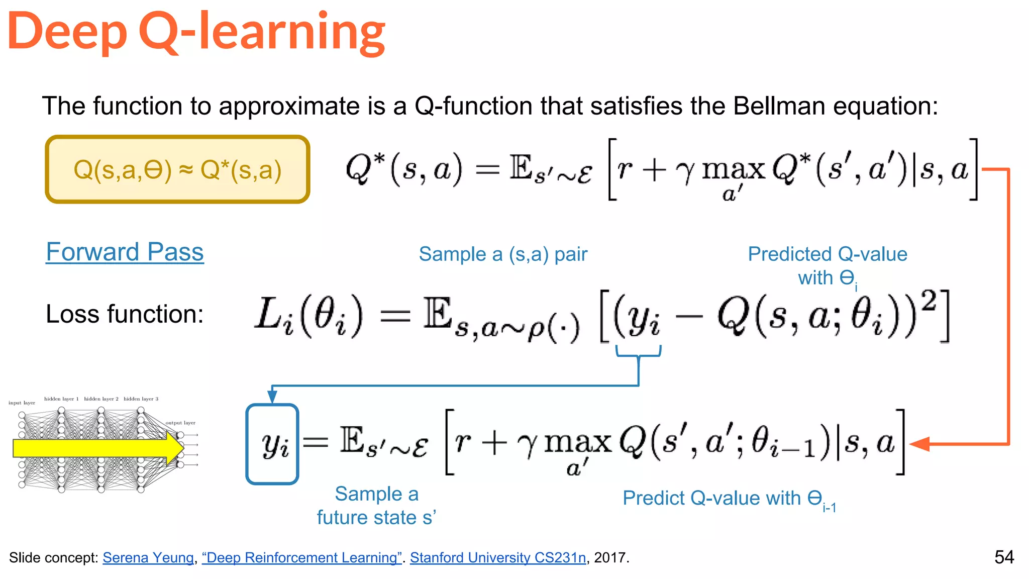
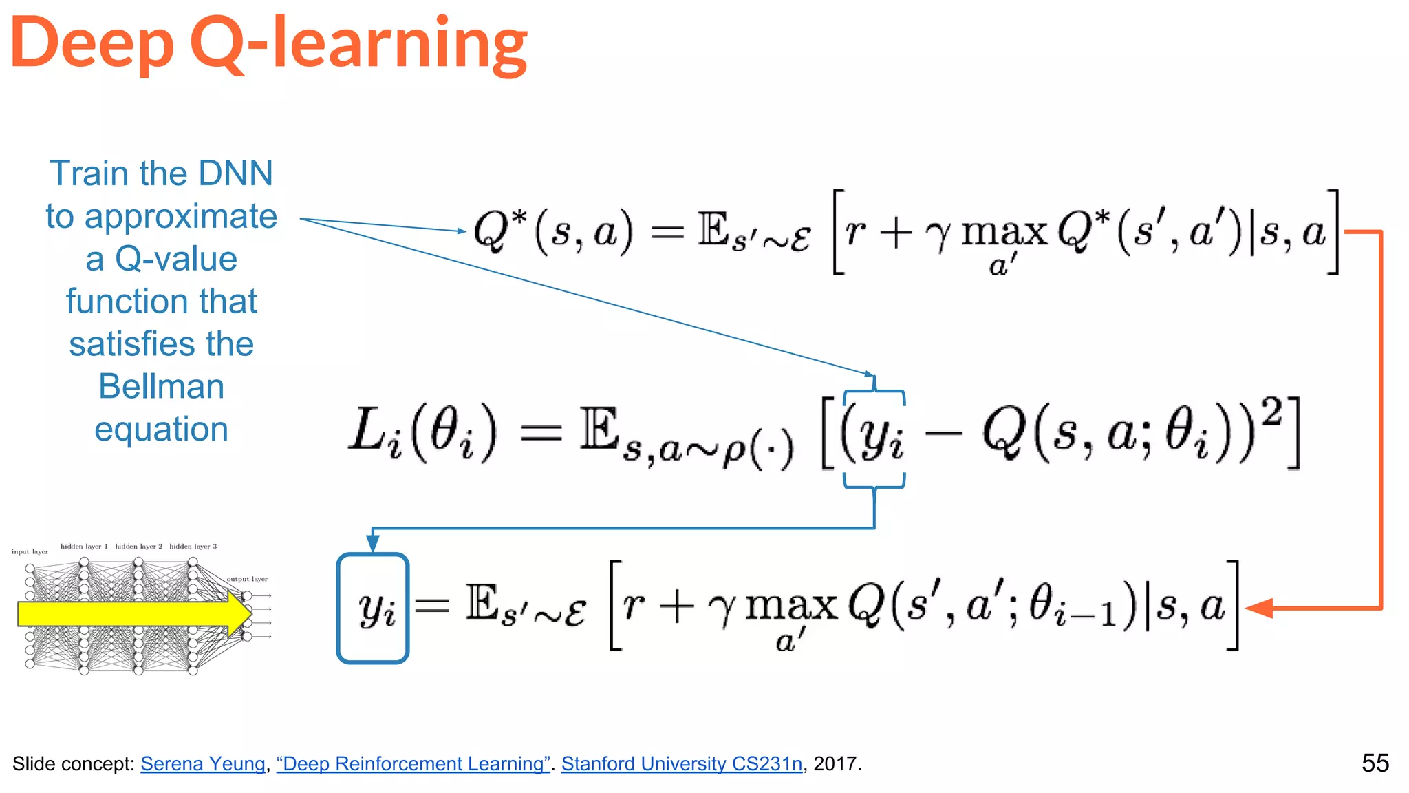
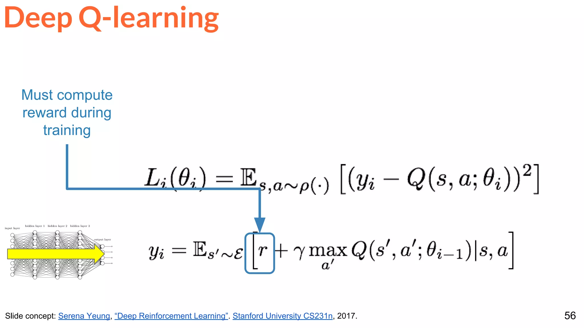
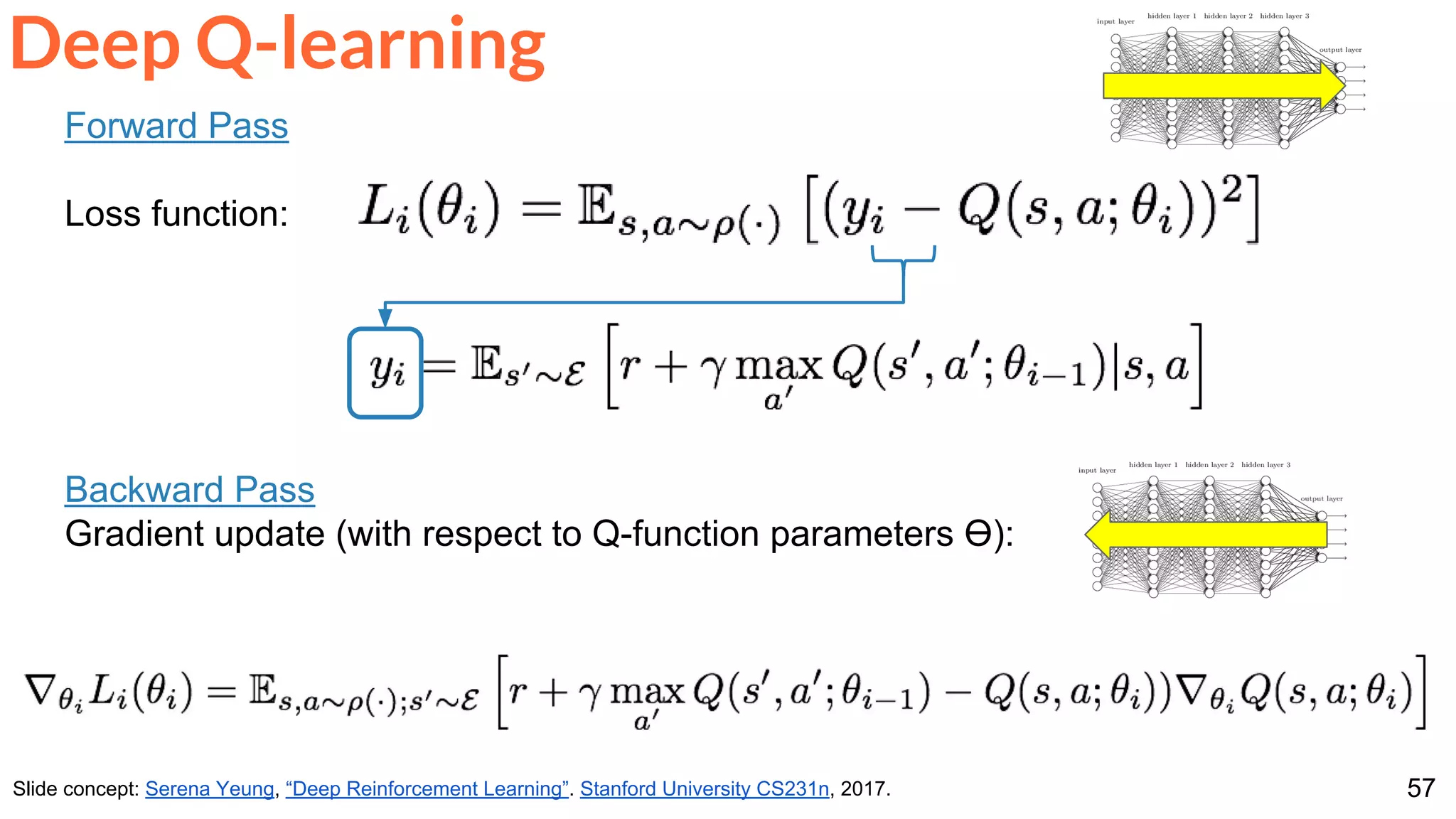
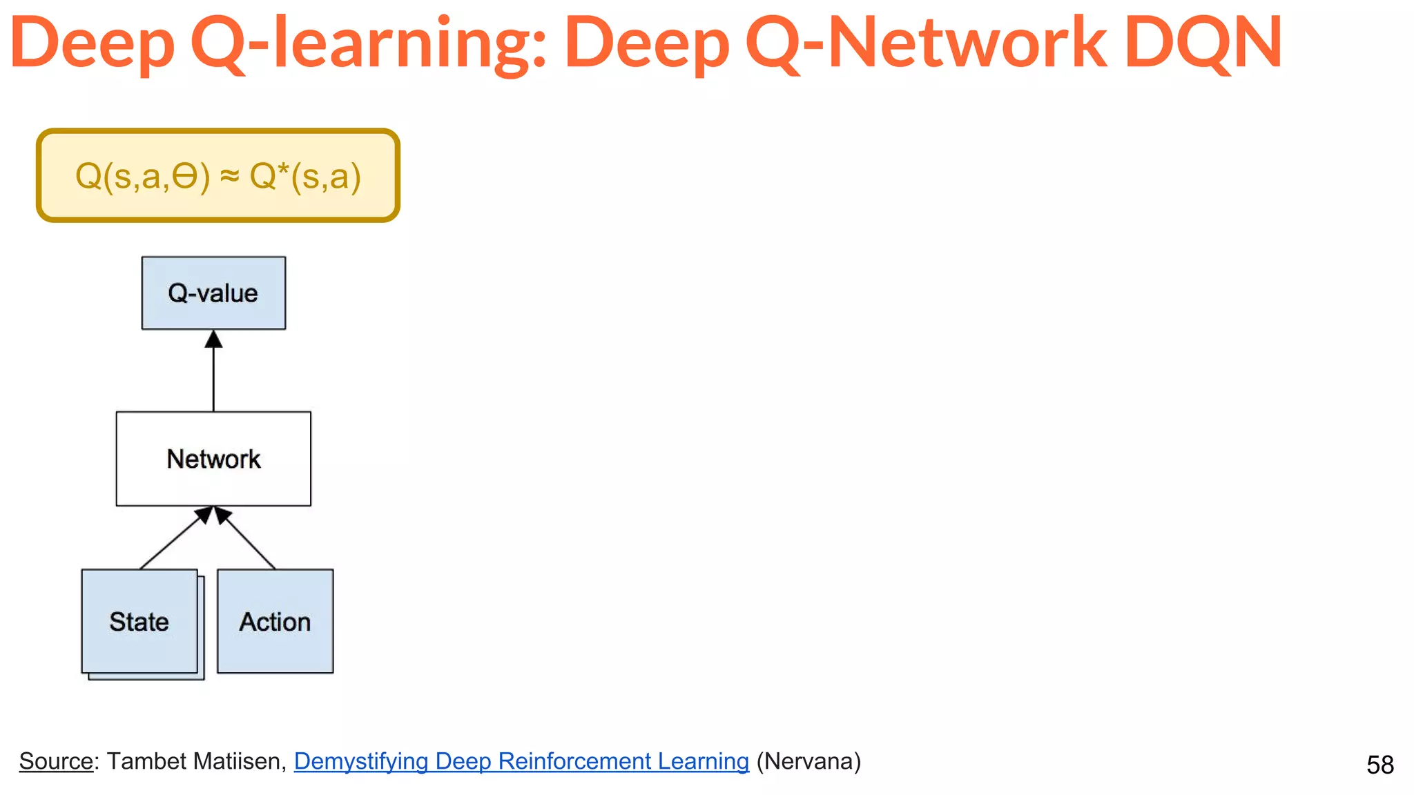
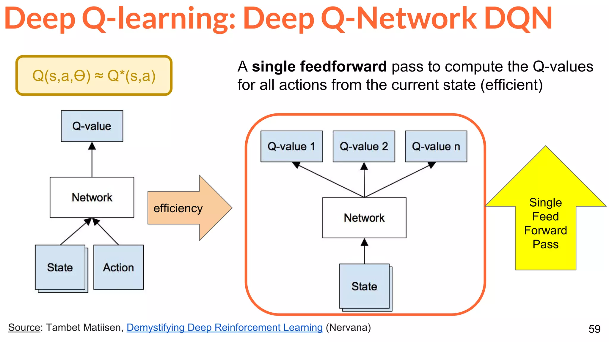
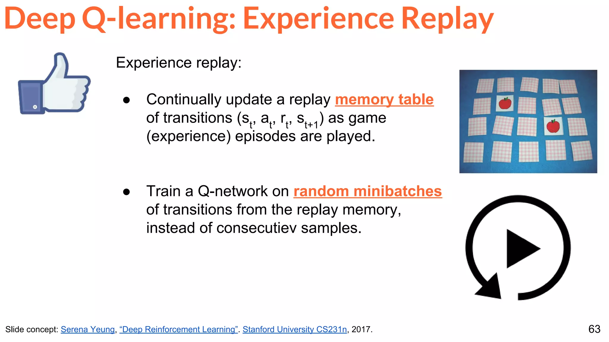
The document is a lecture presentation on reinforcement learning by Xavier Giro-i-Nieto, covering topics such as motivation, architecture, Markov decision processes (MDP), and deep Q-learning techniques. It discusses the categorization of learning procedures, policies, value functions, and the use of deep learning for approximating Q-values. The content also highlights key problems and solutions in reinforcement learning, including experience replay and the application of neural networks.


![[222]대화 시스템 서비스 동향 및 개발 방법](https://cdn.slidesharecdn.com/ss_thumbnails/222-150915011307-lva1-app6892-thumbnail.jpg?width=640&height=640&fit=bounds)


![[DSC Europe 25] Andy Cotgreave - Nothing is new in analytics.pptx](https://cdn.slidesharecdn.com/ss_thumbnails/mba4vzcurvoh5lfrd5zw-6-251205194645-341bbbbe-thumbnail.jpg?width=640&height=640&fit=bounds)


![[DSC Europe 25] Dragan Vucic - Building the Learning Organization - How AI Tr...](https://cdn.slidesharecdn.com/ss_thumbnails/8brigo2sbu6qur6gxrra-7-251205085715-6ae07d24-thumbnail.jpg?width=640&height=640&fit=bounds)
![[DSC Europe 25] Max Talanov - Non digital NNs.pptx](https://cdn.slidesharecdn.com/ss_thumbnails/wif8tr3gtua74qvtopke-non-digital-nns-251205090438-26b0eea6-thumbnail.jpg?width=640&height=640&fit=bounds)


![[DSC Europe 25] Goran Obradovic - The Rise of Sovereign AI: Building the Regi...](https://cdn.slidesharecdn.com/ss_thumbnails/7nw2xxixrxqdxvrb5wca-6-251205085714-ab09a2ac-thumbnail.jpg?width=640&height=640&fit=bounds)

![[DSC Europe 25] Dusan Jovicic - AI Story: From on-prem to cloud and back agai...](https://cdn.slidesharecdn.com/ss_thumbnails/8kp49m6uq22ifnbwhfnk-2-251205085715-964d11a6-thumbnail.jpg?width=640&height=640&fit=bounds)


