This document provides an introduction to reinforcement learning. It defines reinforcement learning as finding a policy that maximizes the sum of rewards by interacting with an environment. It discusses key concepts like Markov decision processes, value functions, temporal difference learning, Q-learning, and deep reinforcement learning. The document also provides examples of applications in games, robotics, economics and comparisons of model-based planning versus model-free reinforcement learning approaches.

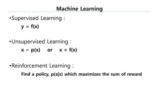
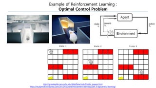
1. Introduction of Reinforcement Learning

2. Artificial Intelligence
• 지능이란?
 보다 추상적인 정보를 이해하는 능력
•인공 지능이란?
 이러한 지능 현상을 인공적으로 구현하려는 연구

3. Artificial Intelligence & Machine Learning

4. Deep Learning in RL
• DeepRL에서 딥러닝은 그저 하나의
module로써만 사용된다.
• Deep Learning의 강점 :
1. 층을 쌓을 수록 더욱 Abstract
Feature Learning이 가능한 유일
한 알고리즘.
2. Universal Function Approximator.

5. Universal Function Approximator

6. Reinforcement Learning이란?

7. •Supervised Learning :
y = f(x)
•Unsupervised Learning :
x ~ p(x) or x = f(x)
•Reinforcement Learning :
Find a policy, p(a|s) which maximizes the sum of reward
Machine Learning

8. Example of Supervised Learning :
Polynomial Curve Fitting
Microsoft Excel 2007의 추세선

9. Example of Unsupervised Learning :
Clustering
http://www.frankichamaki.com/data-driven-market-segmentation-more-effective-marketing-to-segments-using-ai/

10. Example of Reinforcement Learning :
Optimal Control Problem
http://graveleylab.cam.uchc.edu/WebData/mduff/older_papers.html
https://studywolf.wordpress.com/2015/03/29/reinforcement-learning-part-3-egocentric-learning/

11. Markov Decision Processes(MDP)

12. • Discrete state space : S = { A , B }
• State transition probability : P(S’|S) = {PAA = 0.7 , PAB = 0.3 , PBA = 0.5 , PBB = 0.5 }
• Purpose : Finding a steady state distribution
Markov Processes

13. • Discrete state space : S = { A , B }
• State transition probability : P(S’|S) = {PAA = 0.7 , PAB = 0.3 , PBA = 0.5 , PBB = 0.5 }
• Reward function : R(S’=A) = +1 , R(S’=B) = -1
• Purpose : Finding an expected reward distribution
Markov Processes with rewards

14. • Discrete state space : S = { A , B }
• Discrete action space : A = { X, Y }
• (Action conditional) State transition probability : P(S’|S , A) = { … }
• Reward function : R(S’=A) = +1 , R(S’=B) = -1
• Purpose : Finding an optimal policy (maximizes the expected sum of future reward)
Markov Decision Processes

15. •Markov decision processes :
a mathematical framework for modeling decision making.
• MDP are solved via dynamic programming and reinforcement learning.
• Applications : robotics, automated control, economics and manufacturing.
• Examples of MDP :
1) AlphaGo에서는 바둑을 MDP로 정의
2) 자동차 운전을 MDP로 정의
3) 주식시장을 MDP로 정의
Markov Decision Processes

16. • Objective : Finding an optimal policy which maximizes the expected sum of
future rewards
• Algorithms
1) Planning : Exhaustive Search / Dynamic Programming
2) Reinforcement Learning : MC method / TD Learning(Q-learning , …)
Agent-Environment Interaction

17. Discount Factor
• Sum of future rewards in episodic tasks
 Gt := Rt+1 + Rt+2 + Rt+3 + … + RT
• Sum of future rewards in continuous tasks
 Gt := Rt+1 + Rt+2 + Rt+3 + … + RT + …
Gt  ∞ (diverge)
• Sum of discounted future rewards in both case
 Gt := Rt+1 + γRt+2 + γ2Rt+3 + … + γT-1RT + …
= γk−1Rt+k
∞
𝒌=𝟏 (converge)
(Rt is bounded / γ : discount factor, 0 <= γ < 1)

18. Value-based Reinforcement Learning

19. Deterministic Policy, a=f(s)
State S f(S)
A Y
B Y

20. Stochastic Policy, p(a|s)
State S P(X|S) P(Y|S)
A 0.3 0.7
B 0.4 0.6

21. Solution of the MDP : Planning
• So our last job is find optimal policy and there are two approaches.
2) Dynamic Programming
1)Exhaustive Search

22. Find Optimal Policy with Exhaustive Search
If we know the one step dynamics of the
MDP, P(s’,r|s,a) , we can do exhaustive
search iteratively until the end step T.
And we can choose the optimal action
path, but this needs O(N^T)! A
A
(+1)
B
(-1)
A
(+1)
B
(-1)
A
(+1)
B
(-1)
A
(+1)
B
(-1)
A
(+1)
B
(-1)
A
(+1)
B
(-1)
X
X
Y
Y
A
(+1)
B
(-1)
A
(+1)
B
(-1)
A
(+1)
B
(-1)
A
(+1)
B
(-1)

23. Dynamic Programming
• We can apply the DP in this problem, and the computational cost
reduces to O(N2T). (But still we need to know the environment
dynamics.)
• DP is a computer science technique which calculates the final goal
value with compositions of cumulative partial values.

24. • State : 5x5
• Action : 4방향이동
• Reward : A에 도착하면 +10, B에 도착하면 +5, 벽에 부딪히면 -1, 그이외 0
• Discounted Factor : 0.9
Gridworld

25. 1) Policy from state-value function
 One-step ahead search for all actions
with state transition probability(model).
2) Policy from action-value function
 a = f(s) = 𝑎𝑟𝑔𝑚𝑎𝑥 𝑎 𝑞π
𝑠 , 𝑎
Optimal Policy from Value Function

26. Value Function
•We will introduce a value function which let us know the expected
sum of future rewards at given state s.
1) State-value function
2) Action-value function

27. Policy Iteration
•How can we get the state-value function with DP?
(action-value function is similarly computed.)
Policy Iteration = Policy Evaluation + Policy Improvement
27

28. Policy Iteration
28
• Policy iteration consists of
two simultaneous,
interacting processes.
• (policy evaluation)
One making the value
function consistent with the
current policy
• (policy improvement)
And the other making the
policy greedy with respect
to the current value function

29. Policy Iteration
29

30. Solution of the MDP : Learning
•The planning methods must know the perfect dynamics of
environment, P(s’,r|s,a)
•But typically this is really hard to know and empirically impossible.
Therefore we will ignore this term and just calculate the mean of
reward with sampling method. This is the starting point of the
machine learning is embedded.
1) Monte Carlo Methods
2) Temporal-Difference Learning
(some kind of reinforcement learning)
30

31. Monte Carlo Methods
31
Starting State Value
S1 Average of G(S1)
S2 Average of G(S2)
S3 Average of G(S2)
Tabular State-value
function

32. Monte Carlo Methods
32
•We need a full length of experience
for each started state. This is really
time consuming to update one state
while waiting the terminal of episode.

33. Q-learning (Temporal Difference Learning)

34. Temporal-Difference Learning
•TD learning is a combination of Monte Carlo ideas and dynamic
programming (DP) ideas.
•Like Monte Carlo methods, TD methods can learn directly from
raw experience without a model of the environment's dynamics.
•Like DP, TD methods update estimates based in part without
waiting for a final outcome (they bootstrap).
34

35. Bellman Equation
(iterative formulation)

36. Q-learning Algorithm

37. Temporal-Difference Learning
37

38. Temporal-Difference Learning
38

39. On policy / Off policy
• On policy : Target policy = Behavioral policy
there can be only one policy.
 This can learn a stochastic policy. Ex) Q-learning
• Off policy : Target policy != Behavioral policy
there can be several policies.
 Broad applications. Ex) SARSA
39

40. Sarsa: On-Policy TD Control
40

41. Eligibility Trace
41
•Smoothly combine the TD and MC.

42. Eligibility Trace
42

43. Comparisons
43

44. Planning & Learning
•There is only a difference between planning and learning. That is
the existence of model.
•So we call planning is model-based method, and learning is
model-free method.
44

45. Planning + Learning
45

46. Planning vs Learning
• After one-step learning.
46

47. Deep Reinforcement Learning

48. •Value function approximation with deep learning
 Large scale or infinite dimensional state can be solvable
Generalization with deep learning
This needs supervised learning techniques and online moving target regression.

49. Appendix
• Atari 2600 - https://www.youtube.com/watch?v=iqXKQf2BOSE
• Super MARIO - https://www.youtube.com/watch?v=qv6UVOQ0F44
• Robot Learns to Flip Pancakes - https://www.youtube.com/watch?v=W_gxLKSsSIE
• Stanford Autonomous Helicopter - Airshow #2 -
https://www.youtube.com/watch?v=VCdxqn0fcnE
• OpenAI Gym - https://gym.openai.com/envs
• Awesome RL - https://github.com/aikorea/awesome-rl
• Udacity RL course
• TensorFlow DRL - https://github.com/nivwusquorum/tensorflow-deepq
• Karpathy rldemo -
http://cs.stanford.edu/people/karpathy/convnetjs/demo/rldemo.html
49

50. References
[1] Sutton, Richard S., and Andrew G. Barto. Reinforcement learning: An
introduction. MIT press, 1998.
50

51. 감사합니다.