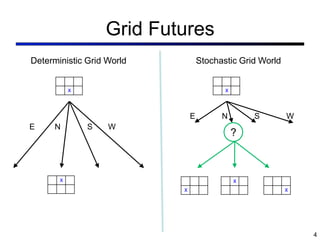
SlideShare a Scribd company logo
Reinforcement
Learning
Slides based on those used in Berkeley's AI class taught by Dan Klein
Reinforcement Learning
 Basic idea:
 Receive feedback in the form of rewards
 Agent’s utility is defined by the reward function
 Must (learn to) act so as to maximize expected rewards
Grid World
 The agent lives in a grid
 Walls block the agent’s path
 The agent’s actions do not always
go as planned:
 80% of the time, the action North
takes the agent North
(if there is no wall there)
 10% of the time, North takes the
agent West; 10% East
 If there is a wall in the direction the
agent would have been taken, the
agent stays put
 Small “living” reward each step
 Big rewards come at the end
 Goal: maximize sum of rewards*
Grid Futures
Deterministic Grid World Stochastic Grid World
X
X
E N S W
X
E N S W
?
X
4
X X
Markov Decision Processes
 An MDP is defined by:
 A set of states s  S
 A set of actions a  A
 A transition function T(s,a,s’)
 Prob that a from s leads to s’
 i.e., P(s’ | s,a)
 Also called the model
 A reward function R(s, a, s’)
 Sometimes just R(s) or R(s’)
 A start state (or distribution)
 Maybe a terminal state
 MDPs are a family of non-
deterministic search problems
 Reinforcement learning: MDPs
where we don’t know the
transition or reward functions
5
Keepaway
6
 http://www.cs.utexas.edu/~AustinVilla/sim/
keepaway/swf/learn360.swf
 SATR
 S0, S0
What is Markov about MDPs?
 Andrey Markov (1856-1922)
 “Markov” generally means that given
the present state, the future and the
past are independent
 For Markov decision processes,
“Markov” means:
Solving MDPs
 In deterministic single-agent search problems, want an
optimal plan, or sequence of actions, from start to a goal
 In an MDP, we want an optimal policy *: S → A
 A policy  gives an action for each state
 An optimal policy maximizes expected utility if followed
 Defines a reflex agent
Optimal policy when
R(s, a, s’) = -0.03 for all
non-terminals s
Example Optimal Policies
R(s) = -2.0
R(s) = -0.4
R(s) = -0.03
R(s) = -0.01
9
MDP Search Trees
 Each MDP state gives an expectimax-like search tree
a
10
s
s’
s, a
(s,a,s’) called a transition
T(s,a,s’) = P(s’|s,a)
R(s,a,s’)
s,a,s’
s is a state
(s, a) is a
q-state
Utilities of Sequences
 In order to formalize optimality of a policy, need to
understand utilities of sequences of rewards
 Typically consider stationary preferences:
 Theorem: only two ways to define stationary utilities
 Additive utility:
 Discounted utility:
11
Infinite Utilities?!
 Problem: infinite state sequences have infinite rewards
 Solutions:
 Finite horizon:
 Terminate episodes after a fixed T steps (e.g. life)
 Gives nonstationary policies ( depends on time left)
 Absorbing state: guarantee that for every policy, a terminal state
will eventually be reached
 Discounting: for 0 < < 1
 Smaller means smaller “horizon” – shorter term focus
12
Discounting
 Typically discount
rewards by < 1
each time step
 Sooner rewards
have higher utility
than later rewards
 Also helps the
algorithms
converge
13
Recap: Defining MDPs
 Markov decision processes:
 States S
0
 Start state s
 Actions A
 Transitions P(s’|s,a) (or T(s,a,s’))
 Rewards R(s,a,s’) (and discount )
 MDP quantities so far:
 Policy = Choice of action for each state
 Utility (or return) = sum of discounted rewards
s
a
s, a
s,a,s’
s’
14
Optimal Utilities
 Fundamental operation: compute
the values (optimal expectimax
utilities) of states s
 Why? Optimal values define
optimal policies!
 Define the value of a state s:
V*(s) = expected utility starting in s
and acting optimally
 Define the value of a q-state (s,a):
Q*(s,a) = expected utility starting in s,
taking action a and thereafter
acting optimally
 Define the optimal policy:
*(s) = optimal action from state s
s
a
s, a
s,a,s’
s’
15
The Bellman Equations
 Definition of “optimal utility” leads to a
simple one-step lookahead relationship
amongst optimal utility values:
Optimal rewards = maximize over first
action and then follow optimal policy
 Formally:
s
a
s, a
s,a,s’
s’
16
Solving MDPs
 We want to find the optimal policy *
 Proposal 1: modified expectimax search, starting from
each state s:
s
a
s, a
s,a,s’
s’
17
Why Not Search Trees?
 Why not solve with expectimax?
 Problems:
 This tree is usually infinite (why?)
 Same states appear over and over (why?)
 We would search once per state (why?)
 Idea: Value iteration
 Compute optimal values for all states all at
once using successive approximations
 Will be a bottom-up dynamic program
similar in cost to memoization
 Do all planning offline, no replanning
needed!
18
Value Estimates
 Calculate estimates V *(s)
k
 Not the optimal value of s!
 The optimal value
considering only next k
time steps (k rewards)
 As k  , it approaches
the optimal value
 Almost solution: recursion
(i.e. expectimax)
 Correct solution: dynamic
programming
19
Value Iteration
 Idea:
 Start with V *(s) = 0, which we know is right (why?)
0
 Given Vi
*, calculate the values for all states for depth i+1:
 This is called a value update or Bellman update
 Repeat until convergence
 Theorem: will converge to unique optimal values
 Basic idea: approximations get refined towards optimal values
 Policy may converge long before values do
20
Example: 
=0.9, living
reward=0, noise=0.2
Example: Bellman Updates
max happens for
a=right, other
actions not shown
21
Example: Value Iteration
 Information propagates outward from terminal
states and eventually all states have correct
value estimates
V2 V3
22
Convergence*
 Define the max-norm:
 Theorem: For any two approximations U and V
 I.e. any distinct approximations must get closer to each other,
so, in particular, any approximation must get closer to the true U
and value iteration converges to a unique, stable, optimal
solution
 Theorem:
 I.e. once the change in our approximation is small, it must also
be close to correct
23
Practice: Computing Actions
 Which action should we chose from state s:
 Given optimal values V?
 Given optimal q-values Q?
 Lesson: actions are easier to select from Q’s!
24
Utilities for Fixed Policies
 Another basic operation: compute
the utility of a state s under a fix
(general non-optimal) policy
 Define the utility of a state s, under a
fixed policy :
V(s) = expected total discounted
rewards (return) starting in s and
following 
 Recursive relation (one-step look-
ahead / Bellman equation):
s
(s)
s, (s)
s, (s),s’
s’
26
Value Iteration
 Idea:
 Start with V *(s) = 0, which we know is right (why?)
0
 Given Vi
*, calculate the values for all states for depth i+1:
 This is called a value update or Bellman update
 Repeat until convergence
 Theorem: will converge to unique optimal values
 Basic idea: approximations get refined towards optimal values
 Policy may converge long before values do
27
Policy Iteration
29
 Problem with value iteration:
 Considering all actions each iteration is slow: takes |A| times longer
than policy evaluation
 But policy doesn’t change each iteration, time wasted
 Alternative to value iteration:
 Step 1: Policy evaluation: calculate utilities for a fixed policy (not optimal
utilities!) until convergence (fast)
 Step 2: Policy improvement: update policy using one-step lookahead
with resulting converged (but not optimal!) utilities (slow but infrequent)
 Repeat steps until policy converges
 This is policy iteration
 It’s still optimal!
 Can converge faster under some conditions
Policy Iteration
 Policy evaluation: with fixed current policy , find values
with simplified Bellman updates:
 Iterate until values converge
 Policy improvement: with fixed utilities, find the best
action according to one-step look-ahead
30
Comparison
31
 In value iteration:
 Every pass (or “backup”) updates both utilities (explicitly, based
on current utilities) and policy (possibly implicitly, based on
current policy)
 In policy iteration:
 Several passes to update utilities with frozen policy
 Occasional passes to update policies
 Hybrid approaches (asynchronous policy iteration):
 Any sequences of partial updates to either policy entries or
utilities will converge if every state is visited infinitely often
Reinforcement Learning
36
 Reinforcement learning:
 Still assume an MDP:
 A set of states s  S
 A set of actions (per state) A
 A model T(s,a,s’)
 A reward function R(s,a,s’)
 Still looking for a policy (s)
 New twist: don’t know T or R
 i.e. don’t know which states are good or what the actions do
 Must actually try actions and states out to learn
Passive Learning
 Simplified task
 You don’t know the transitions T(s,a,s’)
 You don’t know the rewards R(s,a,s’)
 You are given a policy (s)
 Goal: learn the state values
 … what policy evaluation did
 In this case:
 Learner “along for the ride”
 No choice about what actions to take
 Just execute the policy and learn from experience
 We’ll get to the active case soon
 This is NOT offline planning! You actually take actions in the
world and see what happens…
37
Example: Direct Evaluation
 Episodes:
(1,1) up -1
(1,2) up -1
(1,2) up -1
(1,3) right -1
(2,3) right -1
(3,3) right -1
(3,2) up -1
(3,3) right -1
(4,3) exit +100
(done)
x
y
(1,1) up -1
(1,2) up -1
(1,3) right -1
(2,3) right -1
(3,3) right -1
(3,2) up -1
(4,2) exit -100
(done)
V(2,3) ~ (96 + -103) / 2 = -3.5
V(3,3) ~ (99 + 97 + -102) / 3 = 31.3
= 1, R = -1
+100
-100
38
Recap: Model-Based Policy Evaluation
 Simplified Bellman updates to
calculate V for a fixed policy:
 New V is expected one-step-look-
ahead using current V
 Unfortunately, need T and R
s
(s)
s, (s)
s, (s),s’
s’
39
Model-Based Learning
 Idea:
 Learn the model empirically through experience
 Solve for values as if the learned model were correct
 Simple empirical model learning
 Count outcomes for each s,a
 Normalize to give estimate of T(s,a,s’)
 Discover R(s,a,s’) when we experience (s,a,s’)
 Solving the MDP with the learned model
 Iterative policy evaluation, for example
s
(s)
s, (s)
s, (s),s’
s’
40
Example: Model-Based Learning
 Episodes:
(1,1) up -1
(1,2) up -1
(1,2) up -1
(1,3) right -1
(2,3) right -1
(3,3) right -1
(3,2) up -1
(3,3) right -1
(4,3) exit +100
(done)
x
y
T(<3,3>, right, <4,3>) = 1 / 3
T(<2,3>, right, <3,3>) = 2 / 2
+100
-100
41
= 1
(1,1) up -1
(1,2) up -1
(1,3) right -1
(2,3) right -1
(3,3) right -1
(3,2) up -1
(4,2) exit -100
(done)
Model-Free Learning
 Want to compute an expectation weighted by P(x):
 Model-based: estimate P(x) from samples, compute expectation
 Model-free: estimate expectation directly from samples
 Why does this work? Because samples appear with the right
frequencies!
42
Sample-Based Policy Evaluation?
 Who needs T and R? Approximate the
expectation with samples (drawn from T!)
s
(s)
s, (s)
s, (s),s’
s2’ s3’
s1
’’
43
Almost! But we only
actually make progress
when we move to i+1.
Temporal-Difference Learning
 Big idea: learn from every experience!
 Update V(s) each time we experience (s,a,s’,r)
 Likely s’ will contribute updates more often
 Temporal difference learning
 Policy still fixed!
 Move values toward value of whatever
successor occurs: running average!
s
(s)
s, (s)
s’
Sample of V(s):
Update to V(s):
Same update:
44
Exponential Moving Average
 Exponential moving average
 Makes recent samples more important
 Forgets about the past (distant past values were wrong anyway)
 Easy to compute from the running average
 Decreasing learning rate can give converging averages
45
Example: TD Policy Evaluation
T
ake = 1,  = 0.5
(1,1) up -1
(1,2) up -1
(1,2) up -1
(1,3) right -1
(2,3) right -1
(3,3) right -1
(3,2) up -1
(3,3) right -1
(4,3) exit +100
(done)
46
(1,1) up -1
(1,2) up -1
(1,3) right -1
(2,3) right -1
(3,3) right -1
(3,2) up -1
(4,2) exit -100
(done)
Problems with TD Value Learning
 TD value leaning is a model-free way
to do policy evaluation
 However, if we want to turn values into
a (new) policy, we’re sunk:
 Idea: learn Q-values directly
 Makes action selection model-free too!
s
a
s, a
s,a,s’
s’
47
Active Learning
 Full reinforcement learning
 You don’t know the transitions T(s,a,s’)
 You don’t know the rewards R(s,a,s’)
 You can choose any actions you like
 Goal: learn the optimal policy
 … what value iteration did!
 In this case:
 Learner makes choices!
 Fundamental tradeoff: exploration vs. exploitation
 This is NOT offline planning! You actually take actions in the
world and find out what happens…
48
The Story So Far: MDPs and RL
 Compute V*, Q*, * exactly 
 Evaluate a fixed policy 
 If we don’t know the MDP
 We can estimate the MDP then solve
 We can estimate V for a fixed policy 
 We can estimate Q*(s,a) for the
optimal policy while executing an
exploration policy
Value and policy
Iteration
 Policy evaluation
Things we know how to do: Techniques:
 If we know the MDP  Model-based DPs
 Model-based RL
 Model-free RL:
 Value learning
 Q-learning
49
Q-Learning
 Q-Learning: sample-based Q-value iteration
 Learn Q*(s,a) values
 Receive a sample (s,a,s’,r)
 Consider your old estimate:
 Consider your new sample estimate:
 Incorporate the new estimate into a running average:
52
Q-Learning Properties
 Amazing result: Q-learning converges to optimal policy
 If you explore enough
 If you make the learning rate small enough
 … but not decrease it too quickly!
 Basically doesn’t matter how you select actions (!)
 Neat property: off-policy learning
 learn optimal policy without following it (some caveats)
S E S E
53
Exploration / Exploitation
 Several schemes for forcing exploration
 Simplest: random actions ( greedy)
 Every time step, flip a coin
 With probability , act randomly
 With probability 1-, act according to current policy
 Problems with random actions?
 You do explore the space, but keep thrashing
around once learning is done
 One solution: lower  over time
 Another solution: exploration functions
54
Exploration Functions
 When to explore
 Random actions: explore a fixed amount
 Better idea: explore areas whose badness is not (yet)
established
 Exploration function
 Takes a value estimate and a count, and returns an optimistic
utility, e.g. (exact form not important)
55
Q-Learning
 Q-learning produces tables of q-values:
56
Q-Learning
57
 In realistic situations, we cannot possibly learn
about every single state!
 Too many states to visit them all in training
 Too many states to hold the q-tables in memory
 Instead, we want to generalize:
 Learn about some small number of training states
from experience
 Generalize that experience to new, similar states
 This is a fundamental idea in machine learning, and
we’ll see it over and over again
Example: Pacman
 Let’s say we discover
through experience
that this state is bad:
 In naïve q learning, we
know nothing about
this state or its q
states:
 Or even this one!
58
Feature-Based Representations
 Solution: describe a state using
a vector of features
 Features are functions from states
to real numbers (often 0/1) that
capture important properties of the
state
 Example features:
 Distance to closest ghost
 Distance to closest dot
 Number of ghosts
 1 / (dist to dot)2
 Is Pacman in a tunnel? (0/1)
 …… etc.
 Can also describe a q-state (s, a)
with features (e.g. action moves
closer to food)
59
Linear Feature Functions
 Using a feature representation, we can write a
q function (or value function) for any state
using a few weights:
 Advantage: our experience is summed up in a
few powerful numbers
 Disadvantage: states may share features but
be very different in value!
60
Function Approximation
 Q-learning with linear q-functions:
 Intuitive interpretation:
 Adjust weights of active features
 E.g. if something unexpectedly bad happens, disprefer all states
with that state’s features
 Formal justification: online least squares
61
Example: Q-Pacman
62
Policy Search
69
http://heli.stanford.edu/
Policy Search
70
 Problem: often the feature-based policies that work well
aren’t the ones that approximate V / Q best
 E.g. your value functions from project 2 were probably horrible
estimates of future rewards, but they still produced good
decisions
 We’ll see this distinction between modeling and prediction again
later in the course
 Solution: learn the policy that maximizes rewards rather
than the value that predicts rewards
 This is the idea behind policy search, such as what
controlled the upside-down helicopter
Policy Search
71
 Simplest policy search:
 Start with an initial linear value function or q-function
 Nudge each feature weight up and down and see if
your policy is better than before
 Problems:
 How do we tell the policy got better?
 Need to run many sample episodes!
 If there are a lot of features, this can be impractical
Policy Search*
 Advanced policy search:
 Write a stochastic (soft) policy:
 Turns out you can efficiently approximate the
derivative of the returns with respect to the
parameters w (details in the book, but you don’t have
to know them)
 Take uphill steps, recalculate derivatives, etc.
72

More Related Content

Similar to 14_ReinforcementLearning.pptx

Reinforcement Learning
Reinforcement LearningReinforcement Learning
Reinforcement Learning
SVijaylakshmi
 
Head First Reinforcement Learning
Head First Reinforcement LearningHead First Reinforcement Learning
Head First Reinforcement Learning
azzeddine chenine
 
Reinforcement learning
Reinforcement learning Reinforcement learning
Reinforcement learning
Chandra Meena
 
Intro to Reinforcement learning - part I
Intro to Reinforcement learning - part IIntro to Reinforcement learning - part I
Intro to Reinforcement learning - part I
Mikko Mäkipää
 
Reinforcement learning
Reinforcement learningReinforcement learning
Reinforcement learning
Ding Li
 
lecture_21.pptx - PowerPoint Presentation
lecture_21.pptx - PowerPoint Presentationlecture_21.pptx - PowerPoint Presentation
lecture_21.pptx - PowerPoint Presentation
butest
 
POMDP Seminar Backup3
POMDP Seminar Backup3POMDP Seminar Backup3
POMDP Seminar Backup3
Darin Hitchings, Ph.D.
 
Reinforcement learning
Reinforcement learningReinforcement learning
Reinforcement learning
Elias Hasnat
 
RL.ppt
RL.pptRL.ppt
RL.ppt
AzharJamil15
 
Lec2 sampling-based-approximations-and-function-fitting
Lec2 sampling-based-approximations-and-function-fittingLec2 sampling-based-approximations-and-function-fitting
Lec2 sampling-based-approximations-and-function-fitting
Ronald Teo
 
Reinforcement Learning Guide For Beginners
Reinforcement Learning Guide For BeginnersReinforcement Learning Guide For Beginners
Reinforcement Learning Guide For Beginners
gokulprasath06
 
reinforcement-learning its based on the slide of university
reinforcement-learning its based on the slide of universityreinforcement-learning its based on the slide of university
reinforcement-learning its based on the slide of university
MOHDNADEEM971008
 
reinforcement-learning.ppt
reinforcement-learning.pptreinforcement-learning.ppt
reinforcement-learning.ppt
hemalathache
 
Modern Recommendation for Advanced Practitioners part2
Modern Recommendation for Advanced Practitioners part2Modern Recommendation for Advanced Practitioners part2
Modern Recommendation for Advanced Practitioners part2
Flavian Vasile
 
Reinforcement learning, Q-Learning
Reinforcement learning, Q-LearningReinforcement learning, Q-Learning
Reinforcement learning, Q-Learning
Kuppusamy P
 
RL intro
RL introRL intro
RL intro
KhangBom
 
reiniforcement learning.ppt
reiniforcement learning.pptreiniforcement learning.ppt
reiniforcement learning.ppt
charusharma165
 
Matineh Shaker, Artificial Intelligence Scientist, Bonsai at MLconf SF 2017
Matineh Shaker, Artificial Intelligence Scientist, Bonsai at MLconf SF 2017Matineh Shaker, Artificial Intelligence Scientist, Bonsai at MLconf SF 2017
Matineh Shaker, Artificial Intelligence Scientist, Bonsai at MLconf SF 2017
MLconf
 
Andrii Prysiazhnyk: Why the amazon sellers are buiyng the RTX 3080: Dynamic p...
Andrii Prysiazhnyk: Why the amazon sellers are buiyng the RTX 3080: Dynamic p...Andrii Prysiazhnyk: Why the amazon sellers are buiyng the RTX 3080: Dynamic p...
Andrii Prysiazhnyk: Why the amazon sellers are buiyng the RTX 3080: Dynamic p...
Lviv Startup Club
 
Reinforcement-Learning.ppt
Reinforcement-Learning.pptReinforcement-Learning.ppt
Reinforcement-Learning.ppt
Tusharchauhan939328
 

Similar to 14_ReinforcementLearning.pptx (20)

Reinforcement Learning
Reinforcement LearningReinforcement Learning
Reinforcement Learning
 
Head First Reinforcement Learning
Head First Reinforcement LearningHead First Reinforcement Learning
Head First Reinforcement Learning
 
Reinforcement learning
Reinforcement learning Reinforcement learning
Reinforcement learning
 
Intro to Reinforcement learning - part I
Intro to Reinforcement learning - part IIntro to Reinforcement learning - part I
Intro to Reinforcement learning - part I
 
Reinforcement learning
Reinforcement learningReinforcement learning
Reinforcement learning
 
lecture_21.pptx - PowerPoint Presentation
lecture_21.pptx - PowerPoint Presentationlecture_21.pptx - PowerPoint Presentation
lecture_21.pptx - PowerPoint Presentation
 
POMDP Seminar Backup3
POMDP Seminar Backup3POMDP Seminar Backup3
POMDP Seminar Backup3
 
Reinforcement learning
Reinforcement learningReinforcement learning
Reinforcement learning
 
RL.ppt
RL.pptRL.ppt
RL.ppt
 
Lec2 sampling-based-approximations-and-function-fitting
Lec2 sampling-based-approximations-and-function-fittingLec2 sampling-based-approximations-and-function-fitting
Lec2 sampling-based-approximations-and-function-fitting
 
Reinforcement Learning Guide For Beginners
Reinforcement Learning Guide For BeginnersReinforcement Learning Guide For Beginners
Reinforcement Learning Guide For Beginners
 
reinforcement-learning its based on the slide of university
reinforcement-learning its based on the slide of universityreinforcement-learning its based on the slide of university
reinforcement-learning its based on the slide of university
 
reinforcement-learning.ppt
reinforcement-learning.pptreinforcement-learning.ppt
reinforcement-learning.ppt
 
Modern Recommendation for Advanced Practitioners part2
Modern Recommendation for Advanced Practitioners part2Modern Recommendation for Advanced Practitioners part2
Modern Recommendation for Advanced Practitioners part2
 
Reinforcement learning, Q-Learning
Reinforcement learning, Q-LearningReinforcement learning, Q-Learning
Reinforcement learning, Q-Learning
 
RL intro
RL introRL intro
RL intro
 
reiniforcement learning.ppt
reiniforcement learning.pptreiniforcement learning.ppt
reiniforcement learning.ppt
 
Matineh Shaker, Artificial Intelligence Scientist, Bonsai at MLconf SF 2017
Matineh Shaker, Artificial Intelligence Scientist, Bonsai at MLconf SF 2017Matineh Shaker, Artificial Intelligence Scientist, Bonsai at MLconf SF 2017
Matineh Shaker, Artificial Intelligence Scientist, Bonsai at MLconf SF 2017
 
Andrii Prysiazhnyk: Why the amazon sellers are buiyng the RTX 3080: Dynamic p...
Andrii Prysiazhnyk: Why the amazon sellers are buiyng the RTX 3080: Dynamic p...Andrii Prysiazhnyk: Why the amazon sellers are buiyng the RTX 3080: Dynamic p...
Andrii Prysiazhnyk: Why the amazon sellers are buiyng the RTX 3080: Dynamic p...
 
Reinforcement-Learning.ppt
Reinforcement-Learning.pptReinforcement-Learning.ppt
Reinforcement-Learning.ppt
 

More from RithikRaj25

html1.ppt
html1.ppthtml1.ppt
html1.ppt
RithikRaj25
 
Data
DataData
Data
DataData
Introduction To Database.ppt
Introduction To Database.pptIntroduction To Database.ppt
Introduction To Database.ppt
RithikRaj25
 
Data.ppt
Data.pptData.ppt
Data.ppt
RithikRaj25
 
DataTypes.ppt
DataTypes.pptDataTypes.ppt
DataTypes.ppt
RithikRaj25
 
NoSQL.pptx
NoSQL.pptxNoSQL.pptx
NoSQL.pptx
RithikRaj25
 
NoSQL
NoSQLNoSQL
text classification_NB.ppt
text classification_NB.ppttext classification_NB.ppt
text classification_NB.ppt
RithikRaj25
 
html1.ppt
html1.ppthtml1.ppt
html1.ppt
RithikRaj25
 
slide-keras-tf.pptx
slide-keras-tf.pptxslide-keras-tf.pptx
slide-keras-tf.pptx
RithikRaj25
 
Intro_OpenCV.ppt
Intro_OpenCV.pptIntro_OpenCV.ppt
Intro_OpenCV.ppt
RithikRaj25
 
lec1b.ppt
lec1b.pptlec1b.ppt
lec1b.ppt
RithikRaj25
 
PR7.ppt
PR7.pptPR7.ppt
PR7.ppt
RithikRaj25
 
objectdetect_tutorial.ppt
objectdetect_tutorial.pptobjectdetect_tutorial.ppt
objectdetect_tutorial.ppt
RithikRaj25
 
datamining-lect11.pptx
datamining-lect11.pptxdatamining-lect11.pptx
datamining-lect11.pptx
RithikRaj25
 
week6a.ppt
week6a.pptweek6a.ppt
week6a.ppt
RithikRaj25
 

More from RithikRaj25 (17)

html1.ppt
html1.ppthtml1.ppt
html1.ppt
 
Data
DataData
Data
 
Data
DataData
Data
 
Introduction To Database.ppt
Introduction To Database.pptIntroduction To Database.ppt
Introduction To Database.ppt
 
Data.ppt
Data.pptData.ppt
Data.ppt
 
DataTypes.ppt
DataTypes.pptDataTypes.ppt
DataTypes.ppt
 
NoSQL.pptx
NoSQL.pptxNoSQL.pptx
NoSQL.pptx
 
NoSQL
NoSQLNoSQL
NoSQL
 
text classification_NB.ppt
text classification_NB.ppttext classification_NB.ppt
text classification_NB.ppt
 
html1.ppt
html1.ppthtml1.ppt
html1.ppt
 
slide-keras-tf.pptx
slide-keras-tf.pptxslide-keras-tf.pptx
slide-keras-tf.pptx
 
Intro_OpenCV.ppt
Intro_OpenCV.pptIntro_OpenCV.ppt
Intro_OpenCV.ppt
 
lec1b.ppt
lec1b.pptlec1b.ppt
lec1b.ppt
 
PR7.ppt
PR7.pptPR7.ppt
PR7.ppt
 
objectdetect_tutorial.ppt
objectdetect_tutorial.pptobjectdetect_tutorial.ppt
objectdetect_tutorial.ppt
 
datamining-lect11.pptx
datamining-lect11.pptxdatamining-lect11.pptx
datamining-lect11.pptx
 
week6a.ppt
week6a.pptweek6a.ppt
week6a.ppt
 

Recently uploaded

Predictably Improve Your B2B Tech Company's Performance by Leveraging Data
Predictably Improve Your B2B Tech Company's Performance by Leveraging DataPredictably Improve Your B2B Tech Company's Performance by Leveraging Data
Predictably Improve Your B2B Tech Company's Performance by Leveraging Data
Kiwi Creative
 
一比一原版(Unimelb毕业证书)墨尔本大学毕业证如何办理
一比一原版(Unimelb毕业证书)墨尔本大学毕业证如何办理一比一原版(Unimelb毕业证书)墨尔本大学毕业证如何办理
一比一原版(Unimelb毕业证书)墨尔本大学毕业证如何办理
xclpvhuk
 
06-12-2024-BudapestDataForum-BuildingReal-timePipelineswithFLaNK AIM
06-12-2024-BudapestDataForum-BuildingReal-timePipelineswithFLaNK AIM06-12-2024-BudapestDataForum-BuildingReal-timePipelineswithFLaNK AIM
06-12-2024-BudapestDataForum-BuildingReal-timePipelineswithFLaNK AIM
Timothy Spann
 
Population Growth in Bataan: The effects of population growth around rural pl...
Population Growth in Bataan: The effects of population growth around rural pl...Population Growth in Bataan: The effects of population growth around rural pl...
Population Growth in Bataan: The effects of population growth around rural pl...
Bill641377
 
Learn SQL from basic queries to Advance queries
Learn SQL from basic queries to Advance queriesLearn SQL from basic queries to Advance queries
Learn SQL from basic queries to Advance queries
manishkhaire30
 
Analysis insight about a Flyball dog competition team's performance
Analysis insight about a Flyball dog competition team's performanceAnalysis insight about a Flyball dog competition team's performance
Analysis insight about a Flyball dog competition team's performance
roli9797
 
Open Source Contributions to Postgres: The Basics POSETTE 2024
Open Source Contributions to Postgres: The Basics POSETTE 2024Open Source Contributions to Postgres: The Basics POSETTE 2024
Open Source Contributions to Postgres: The Basics POSETTE 2024
ElizabethGarrettChri
 
DSSML24_tspann_CodelessGenerativeAIPipelines
DSSML24_tspann_CodelessGenerativeAIPipelinesDSSML24_tspann_CodelessGenerativeAIPipelines
DSSML24_tspann_CodelessGenerativeAIPipelines
Timothy Spann
 
STATATHON: Unleashing the Power of Statistics in a 48-Hour Knowledge Extravag...
STATATHON: Unleashing the Power of Statistics in a 48-Hour Knowledge Extravag...STATATHON: Unleashing the Power of Statistics in a 48-Hour Knowledge Extravag...
STATATHON: Unleashing the Power of Statistics in a 48-Hour Knowledge Extravag...
sameer shah
 
Palo Alto Cortex XDR presentation .......
Palo Alto Cortex XDR presentation .......Palo Alto Cortex XDR presentation .......
Palo Alto Cortex XDR presentation .......
Sachin Paul
 
一比一原版(UMN文凭证书)明尼苏达大学毕业证如何办理
一比一原版(UMN文凭证书)明尼苏达大学毕业证如何办理一比一原版(UMN文凭证书)明尼苏达大学毕业证如何办理
一比一原版(UMN文凭证书)明尼苏达大学毕业证如何办理
nyfuhyz
 
在线办理(英国UCA毕业证书)创意艺术大学毕业证在读证明一模一样
在线办理(英国UCA毕业证书)创意艺术大学毕业证在读证明一模一样在线办理(英国UCA毕业证书)创意艺术大学毕业证在读证明一模一样
在线办理(英国UCA毕业证书)创意艺术大学毕业证在读证明一模一样
v7oacc3l
 
原版一比一利兹贝克特大学毕业证(LeedsBeckett毕业证书)如何办理
原版一比一利兹贝克特大学毕业证(LeedsBeckett毕业证书)如何办理原版一比一利兹贝克特大学毕业证(LeedsBeckett毕业证书)如何办理
原版一比一利兹贝克特大学毕业证(LeedsBeckett毕业证书)如何办理
wyddcwye1
 
一比一原版(UO毕业证)渥太华大学毕业证如何办理
一比一原版(UO毕业证)渥太华大学毕业证如何办理一比一原版(UO毕业证)渥太华大学毕业证如何办理
一比一原版(UO毕业证)渥太华大学毕业证如何办理
aqzctr7x
 
A presentation that explain the Power BI Licensing
A presentation that explain the Power BI LicensingA presentation that explain the Power BI Licensing
A presentation that explain the Power BI Licensing
AlessioFois2
 
Everything you wanted to know about LIHTC
Everything you wanted to know about LIHTCEverything you wanted to know about LIHTC
Everything you wanted to know about LIHTC
Roger Valdez
 
原版制作(unimelb毕业证书)墨尔本大学毕业证Offer一模一样
原版制作(unimelb毕业证书)墨尔本大学毕业证Offer一模一样原版制作(unimelb毕业证书)墨尔本大学毕业证Offer一模一样
原版制作(unimelb毕业证书)墨尔本大学毕业证Offer一模一样
ihavuls
 
DATA COMMS-NETWORKS YR2 lecture 08 NAT & CLOUD.docx
DATA COMMS-NETWORKS YR2 lecture 08 NAT & CLOUD.docxDATA COMMS-NETWORKS YR2 lecture 08 NAT & CLOUD.docx
DATA COMMS-NETWORKS YR2 lecture 08 NAT & CLOUD.docx
SaffaIbrahim1
 
ViewShift: Hassle-free Dynamic Policy Enforcement for Every Data Lake
ViewShift: Hassle-free Dynamic Policy Enforcement for Every Data LakeViewShift: Hassle-free Dynamic Policy Enforcement for Every Data Lake
ViewShift: Hassle-free Dynamic Policy Enforcement for Every Data Lake
Walaa Eldin Moustafa
 
University of New South Wales degree offer diploma Transcript
University of New South Wales degree offer diploma TranscriptUniversity of New South Wales degree offer diploma Transcript
University of New South Wales degree offer diploma Transcript
soxrziqu
 

Recently uploaded (20)

Predictably Improve Your B2B Tech Company's Performance by Leveraging Data
Predictably Improve Your B2B Tech Company's Performance by Leveraging DataPredictably Improve Your B2B Tech Company's Performance by Leveraging Data
Predictably Improve Your B2B Tech Company's Performance by Leveraging Data
 
一比一原版(Unimelb毕业证书)墨尔本大学毕业证如何办理
一比一原版(Unimelb毕业证书)墨尔本大学毕业证如何办理一比一原版(Unimelb毕业证书)墨尔本大学毕业证如何办理
一比一原版(Unimelb毕业证书)墨尔本大学毕业证如何办理
 
06-12-2024-BudapestDataForum-BuildingReal-timePipelineswithFLaNK AIM
06-12-2024-BudapestDataForum-BuildingReal-timePipelineswithFLaNK AIM06-12-2024-BudapestDataForum-BuildingReal-timePipelineswithFLaNK AIM
06-12-2024-BudapestDataForum-BuildingReal-timePipelineswithFLaNK AIM
 
Population Growth in Bataan: The effects of population growth around rural pl...
Population Growth in Bataan: The effects of population growth around rural pl...Population Growth in Bataan: The effects of population growth around rural pl...
Population Growth in Bataan: The effects of population growth around rural pl...
 
Learn SQL from basic queries to Advance queries
Learn SQL from basic queries to Advance queriesLearn SQL from basic queries to Advance queries
Learn SQL from basic queries to Advance queries
 
Analysis insight about a Flyball dog competition team's performance
Analysis insight about a Flyball dog competition team's performanceAnalysis insight about a Flyball dog competition team's performance
Analysis insight about a Flyball dog competition team's performance
 
Open Source Contributions to Postgres: The Basics POSETTE 2024
Open Source Contributions to Postgres: The Basics POSETTE 2024Open Source Contributions to Postgres: The Basics POSETTE 2024
Open Source Contributions to Postgres: The Basics POSETTE 2024
 
DSSML24_tspann_CodelessGenerativeAIPipelines
DSSML24_tspann_CodelessGenerativeAIPipelinesDSSML24_tspann_CodelessGenerativeAIPipelines
DSSML24_tspann_CodelessGenerativeAIPipelines
 
STATATHON: Unleashing the Power of Statistics in a 48-Hour Knowledge Extravag...
STATATHON: Unleashing the Power of Statistics in a 48-Hour Knowledge Extravag...STATATHON: Unleashing the Power of Statistics in a 48-Hour Knowledge Extravag...
STATATHON: Unleashing the Power of Statistics in a 48-Hour Knowledge Extravag...
 
Palo Alto Cortex XDR presentation .......
Palo Alto Cortex XDR presentation .......Palo Alto Cortex XDR presentation .......
Palo Alto Cortex XDR presentation .......
 
一比一原版(UMN文凭证书)明尼苏达大学毕业证如何办理
一比一原版(UMN文凭证书)明尼苏达大学毕业证如何办理一比一原版(UMN文凭证书)明尼苏达大学毕业证如何办理
一比一原版(UMN文凭证书)明尼苏达大学毕业证如何办理
 
在线办理(英国UCA毕业证书)创意艺术大学毕业证在读证明一模一样
在线办理(英国UCA毕业证书)创意艺术大学毕业证在读证明一模一样在线办理(英国UCA毕业证书)创意艺术大学毕业证在读证明一模一样
在线办理(英国UCA毕业证书)创意艺术大学毕业证在读证明一模一样
 
原版一比一利兹贝克特大学毕业证(LeedsBeckett毕业证书)如何办理
原版一比一利兹贝克特大学毕业证(LeedsBeckett毕业证书)如何办理原版一比一利兹贝克特大学毕业证(LeedsBeckett毕业证书)如何办理
原版一比一利兹贝克特大学毕业证(LeedsBeckett毕业证书)如何办理
 
一比一原版(UO毕业证)渥太华大学毕业证如何办理
一比一原版(UO毕业证)渥太华大学毕业证如何办理一比一原版(UO毕业证)渥太华大学毕业证如何办理
一比一原版(UO毕业证)渥太华大学毕业证如何办理
 
A presentation that explain the Power BI Licensing
A presentation that explain the Power BI LicensingA presentation that explain the Power BI Licensing
A presentation that explain the Power BI Licensing
 
Everything you wanted to know about LIHTC
Everything you wanted to know about LIHTCEverything you wanted to know about LIHTC
Everything you wanted to know about LIHTC
 
原版制作(unimelb毕业证书)墨尔本大学毕业证Offer一模一样
原版制作(unimelb毕业证书)墨尔本大学毕业证Offer一模一样原版制作(unimelb毕业证书)墨尔本大学毕业证Offer一模一样
原版制作(unimelb毕业证书)墨尔本大学毕业证Offer一模一样
 
DATA COMMS-NETWORKS YR2 lecture 08 NAT & CLOUD.docx
DATA COMMS-NETWORKS YR2 lecture 08 NAT & CLOUD.docxDATA COMMS-NETWORKS YR2 lecture 08 NAT & CLOUD.docx
DATA COMMS-NETWORKS YR2 lecture 08 NAT & CLOUD.docx
 
ViewShift: Hassle-free Dynamic Policy Enforcement for Every Data Lake
ViewShift: Hassle-free Dynamic Policy Enforcement for Every Data LakeViewShift: Hassle-free Dynamic Policy Enforcement for Every Data Lake
ViewShift: Hassle-free Dynamic Policy Enforcement for Every Data Lake
 
University of New South Wales degree offer diploma Transcript
University of New South Wales degree offer diploma TranscriptUniversity of New South Wales degree offer diploma Transcript
University of New South Wales degree offer diploma Transcript
 

14_ReinforcementLearning.pptx

  • 1. Reinforcement Learning Slides based on those used in Berkeley's AI class taught by Dan Klein
  • 2. Reinforcement Learning  Basic idea:  Receive feedback in the form of rewards  Agent’s utility is defined by the reward function  Must (learn to) act so as to maximize expected rewards
  • 3. Grid World  The agent lives in a grid  Walls block the agent’s path  The agent’s actions do not always go as planned:  80% of the time, the action North takes the agent North (if there is no wall there)  10% of the time, North takes the agent West; 10% East  If there is a wall in the direction the agent would have been taken, the agent stays put  Small “living” reward each step  Big rewards come at the end  Goal: maximize sum of rewards*
  • 4. Grid Futures Deterministic Grid World Stochastic Grid World X X E N S W X E N S W ? X 4 X X
  • 5. Markov Decision Processes  An MDP is defined by:  A set of states s  S  A set of actions a  A  A transition function T(s,a,s’)  Prob that a from s leads to s’  i.e., P(s’ | s,a)  Also called the model  A reward function R(s, a, s’)  Sometimes just R(s) or R(s’)  A start state (or distribution)  Maybe a terminal state  MDPs are a family of non- deterministic search problems  Reinforcement learning: MDPs where we don’t know the transition or reward functions 5
  • 7. What is Markov about MDPs?  Andrey Markov (1856-1922)  “Markov” generally means that given the present state, the future and the past are independent  For Markov decision processes, “Markov” means:
  • 8. Solving MDPs  In deterministic single-agent search problems, want an optimal plan, or sequence of actions, from start to a goal  In an MDP, we want an optimal policy *: S → A  A policy  gives an action for each state  An optimal policy maximizes expected utility if followed  Defines a reflex agent Optimal policy when R(s, a, s’) = -0.03 for all non-terminals s
  • 9. Example Optimal Policies R(s) = -2.0 R(s) = -0.4 R(s) = -0.03 R(s) = -0.01 9
  • 10. MDP Search Trees  Each MDP state gives an expectimax-like search tree a 10 s s’ s, a (s,a,s’) called a transition T(s,a,s’) = P(s’|s,a) R(s,a,s’) s,a,s’ s is a state (s, a) is a q-state
  • 11. Utilities of Sequences  In order to formalize optimality of a policy, need to understand utilities of sequences of rewards  Typically consider stationary preferences:  Theorem: only two ways to define stationary utilities  Additive utility:  Discounted utility: 11
  • 12. Infinite Utilities?!  Problem: infinite state sequences have infinite rewards  Solutions:  Finite horizon:  Terminate episodes after a fixed T steps (e.g. life)  Gives nonstationary policies ( depends on time left)  Absorbing state: guarantee that for every policy, a terminal state will eventually be reached  Discounting: for 0 < < 1  Smaller means smaller “horizon” – shorter term focus 12
  • 13. Discounting  Typically discount rewards by < 1 each time step  Sooner rewards have higher utility than later rewards  Also helps the algorithms converge 13
  • 14. Recap: Defining MDPs  Markov decision processes:  States S 0  Start state s  Actions A  Transitions P(s’|s,a) (or T(s,a,s’))  Rewards R(s,a,s’) (and discount )  MDP quantities so far:  Policy = Choice of action for each state  Utility (or return) = sum of discounted rewards s a s, a s,a,s’ s’ 14
  • 15. Optimal Utilities  Fundamental operation: compute the values (optimal expectimax utilities) of states s  Why? Optimal values define optimal policies!  Define the value of a state s: V*(s) = expected utility starting in s and acting optimally  Define the value of a q-state (s,a): Q*(s,a) = expected utility starting in s, taking action a and thereafter acting optimally  Define the optimal policy: *(s) = optimal action from state s s a s, a s,a,s’ s’ 15
  • 16. The Bellman Equations  Definition of “optimal utility” leads to a simple one-step lookahead relationship amongst optimal utility values: Optimal rewards = maximize over first action and then follow optimal policy  Formally: s a s, a s,a,s’ s’ 16
  • 17. Solving MDPs  We want to find the optimal policy *  Proposal 1: modified expectimax search, starting from each state s: s a s, a s,a,s’ s’ 17
  • 18. Why Not Search Trees?  Why not solve with expectimax?  Problems:  This tree is usually infinite (why?)  Same states appear over and over (why?)  We would search once per state (why?)  Idea: Value iteration  Compute optimal values for all states all at once using successive approximations  Will be a bottom-up dynamic program similar in cost to memoization  Do all planning offline, no replanning needed! 18
  • 19. Value Estimates  Calculate estimates V *(s) k  Not the optimal value of s!  The optimal value considering only next k time steps (k rewards)  As k  , it approaches the optimal value  Almost solution: recursion (i.e. expectimax)  Correct solution: dynamic programming 19
  • 20. Value Iteration  Idea:  Start with V *(s) = 0, which we know is right (why?) 0  Given Vi *, calculate the values for all states for depth i+1:  This is called a value update or Bellman update  Repeat until convergence  Theorem: will converge to unique optimal values  Basic idea: approximations get refined towards optimal values  Policy may converge long before values do 20
  • 21. Example:  =0.9, living reward=0, noise=0.2 Example: Bellman Updates max happens for a=right, other actions not shown 21
  • 22. Example: Value Iteration  Information propagates outward from terminal states and eventually all states have correct value estimates V2 V3 22
  • 23. Convergence*  Define the max-norm:  Theorem: For any two approximations U and V  I.e. any distinct approximations must get closer to each other, so, in particular, any approximation must get closer to the true U and value iteration converges to a unique, stable, optimal solution  Theorem:  I.e. once the change in our approximation is small, it must also be close to correct 23
  • 24. Practice: Computing Actions  Which action should we chose from state s:  Given optimal values V?  Given optimal q-values Q?  Lesson: actions are easier to select from Q’s! 24
  • 25. Utilities for Fixed Policies  Another basic operation: compute the utility of a state s under a fix (general non-optimal) policy  Define the utility of a state s, under a fixed policy : V(s) = expected total discounted rewards (return) starting in s and following   Recursive relation (one-step look- ahead / Bellman equation): s (s) s, (s) s, (s),s’ s’ 26
  • 26. Value Iteration  Idea:  Start with V *(s) = 0, which we know is right (why?) 0  Given Vi *, calculate the values for all states for depth i+1:  This is called a value update or Bellman update  Repeat until convergence  Theorem: will converge to unique optimal values  Basic idea: approximations get refined towards optimal values  Policy may converge long before values do 27
  • 27. Policy Iteration 29  Problem with value iteration:  Considering all actions each iteration is slow: takes |A| times longer than policy evaluation  But policy doesn’t change each iteration, time wasted  Alternative to value iteration:  Step 1: Policy evaluation: calculate utilities for a fixed policy (not optimal utilities!) until convergence (fast)  Step 2: Policy improvement: update policy using one-step lookahead with resulting converged (but not optimal!) utilities (slow but infrequent)  Repeat steps until policy converges  This is policy iteration  It’s still optimal!  Can converge faster under some conditions
  • 28. Policy Iteration  Policy evaluation: with fixed current policy , find values with simplified Bellman updates:  Iterate until values converge  Policy improvement: with fixed utilities, find the best action according to one-step look-ahead 30
  • 29. Comparison 31  In value iteration:  Every pass (or “backup”) updates both utilities (explicitly, based on current utilities) and policy (possibly implicitly, based on current policy)  In policy iteration:  Several passes to update utilities with frozen policy  Occasional passes to update policies  Hybrid approaches (asynchronous policy iteration):  Any sequences of partial updates to either policy entries or utilities will converge if every state is visited infinitely often
  • 30. Reinforcement Learning 36  Reinforcement learning:  Still assume an MDP:  A set of states s  S  A set of actions (per state) A  A model T(s,a,s’)  A reward function R(s,a,s’)  Still looking for a policy (s)  New twist: don’t know T or R  i.e. don’t know which states are good or what the actions do  Must actually try actions and states out to learn
  • 31. Passive Learning  Simplified task  You don’t know the transitions T(s,a,s’)  You don’t know the rewards R(s,a,s’)  You are given a policy (s)  Goal: learn the state values  … what policy evaluation did  In this case:  Learner “along for the ride”  No choice about what actions to take  Just execute the policy and learn from experience  We’ll get to the active case soon  This is NOT offline planning! You actually take actions in the world and see what happens… 37
  • 32. Example: Direct Evaluation  Episodes: (1,1) up -1 (1,2) up -1 (1,2) up -1 (1,3) right -1 (2,3) right -1 (3,3) right -1 (3,2) up -1 (3,3) right -1 (4,3) exit +100 (done) x y (1,1) up -1 (1,2) up -1 (1,3) right -1 (2,3) right -1 (3,3) right -1 (3,2) up -1 (4,2) exit -100 (done) V(2,3) ~ (96 + -103) / 2 = -3.5 V(3,3) ~ (99 + 97 + -102) / 3 = 31.3 = 1, R = -1 +100 -100 38
  • 33. Recap: Model-Based Policy Evaluation  Simplified Bellman updates to calculate V for a fixed policy:  New V is expected one-step-look- ahead using current V  Unfortunately, need T and R s (s) s, (s) s, (s),s’ s’ 39
  • 34. Model-Based Learning  Idea:  Learn the model empirically through experience  Solve for values as if the learned model were correct  Simple empirical model learning  Count outcomes for each s,a  Normalize to give estimate of T(s,a,s’)  Discover R(s,a,s’) when we experience (s,a,s’)  Solving the MDP with the learned model  Iterative policy evaluation, for example s (s) s, (s) s, (s),s’ s’ 40
  • 35. Example: Model-Based Learning  Episodes: (1,1) up -1 (1,2) up -1 (1,2) up -1 (1,3) right -1 (2,3) right -1 (3,3) right -1 (3,2) up -1 (3,3) right -1 (4,3) exit +100 (done) x y T(<3,3>, right, <4,3>) = 1 / 3 T(<2,3>, right, <3,3>) = 2 / 2 +100 -100 41 = 1 (1,1) up -1 (1,2) up -1 (1,3) right -1 (2,3) right -1 (3,3) right -1 (3,2) up -1 (4,2) exit -100 (done)
  • 36. Model-Free Learning  Want to compute an expectation weighted by P(x):  Model-based: estimate P(x) from samples, compute expectation  Model-free: estimate expectation directly from samples  Why does this work? Because samples appear with the right frequencies! 42
  • 37. Sample-Based Policy Evaluation?  Who needs T and R? Approximate the expectation with samples (drawn from T!) s (s) s, (s) s, (s),s’ s2’ s3’ s1 ’’ 43 Almost! But we only actually make progress when we move to i+1.
  • 38. Temporal-Difference Learning  Big idea: learn from every experience!  Update V(s) each time we experience (s,a,s’,r)  Likely s’ will contribute updates more often  Temporal difference learning  Policy still fixed!  Move values toward value of whatever successor occurs: running average! s (s) s, (s) s’ Sample of V(s): Update to V(s): Same update: 44
  • 39. Exponential Moving Average  Exponential moving average  Makes recent samples more important  Forgets about the past (distant past values were wrong anyway)  Easy to compute from the running average  Decreasing learning rate can give converging averages 45
  • 40. Example: TD Policy Evaluation T ake = 1,  = 0.5 (1,1) up -1 (1,2) up -1 (1,2) up -1 (1,3) right -1 (2,3) right -1 (3,3) right -1 (3,2) up -1 (3,3) right -1 (4,3) exit +100 (done) 46 (1,1) up -1 (1,2) up -1 (1,3) right -1 (2,3) right -1 (3,3) right -1 (3,2) up -1 (4,2) exit -100 (done)
  • 41. Problems with TD Value Learning  TD value leaning is a model-free way to do policy evaluation  However, if we want to turn values into a (new) policy, we’re sunk:  Idea: learn Q-values directly  Makes action selection model-free too! s a s, a s,a,s’ s’ 47
  • 42. Active Learning  Full reinforcement learning  You don’t know the transitions T(s,a,s’)  You don’t know the rewards R(s,a,s’)  You can choose any actions you like  Goal: learn the optimal policy  … what value iteration did!  In this case:  Learner makes choices!  Fundamental tradeoff: exploration vs. exploitation  This is NOT offline planning! You actually take actions in the world and find out what happens… 48
  • 43. The Story So Far: MDPs and RL  Compute V*, Q*, * exactly   Evaluate a fixed policy   If we don’t know the MDP  We can estimate the MDP then solve  We can estimate V for a fixed policy   We can estimate Q*(s,a) for the optimal policy while executing an exploration policy Value and policy Iteration  Policy evaluation Things we know how to do: Techniques:  If we know the MDP  Model-based DPs  Model-based RL  Model-free RL:  Value learning  Q-learning 49
  • 44. Q-Learning  Q-Learning: sample-based Q-value iteration  Learn Q*(s,a) values  Receive a sample (s,a,s’,r)  Consider your old estimate:  Consider your new sample estimate:  Incorporate the new estimate into a running average: 52
  • 45. Q-Learning Properties  Amazing result: Q-learning converges to optimal policy  If you explore enough  If you make the learning rate small enough  … but not decrease it too quickly!  Basically doesn’t matter how you select actions (!)  Neat property: off-policy learning  learn optimal policy without following it (some caveats) S E S E 53
  • 46. Exploration / Exploitation  Several schemes for forcing exploration  Simplest: random actions ( greedy)  Every time step, flip a coin  With probability , act randomly  With probability 1-, act according to current policy  Problems with random actions?  You do explore the space, but keep thrashing around once learning is done  One solution: lower  over time  Another solution: exploration functions 54
  • 47. Exploration Functions  When to explore  Random actions: explore a fixed amount  Better idea: explore areas whose badness is not (yet) established  Exploration function  Takes a value estimate and a count, and returns an optimistic utility, e.g. (exact form not important) 55
  • 48. Q-Learning  Q-learning produces tables of q-values: 56
  • 49. Q-Learning 57  In realistic situations, we cannot possibly learn about every single state!  Too many states to visit them all in training  Too many states to hold the q-tables in memory  Instead, we want to generalize:  Learn about some small number of training states from experience  Generalize that experience to new, similar states  This is a fundamental idea in machine learning, and we’ll see it over and over again
  • 50. Example: Pacman  Let’s say we discover through experience that this state is bad:  In naïve q learning, we know nothing about this state or its q states:  Or even this one! 58
  • 51. Feature-Based Representations  Solution: describe a state using a vector of features  Features are functions from states to real numbers (often 0/1) that capture important properties of the state  Example features:  Distance to closest ghost  Distance to closest dot  Number of ghosts  1 / (dist to dot)2  Is Pacman in a tunnel? (0/1)  …… etc.  Can also describe a q-state (s, a) with features (e.g. action moves closer to food) 59
  • 52. Linear Feature Functions  Using a feature representation, we can write a q function (or value function) for any state using a few weights:  Advantage: our experience is summed up in a few powerful numbers  Disadvantage: states may share features but be very different in value! 60
  • 53. Function Approximation  Q-learning with linear q-functions:  Intuitive interpretation:  Adjust weights of active features  E.g. if something unexpectedly bad happens, disprefer all states with that state’s features  Formal justification: online least squares 61
  • 56. Policy Search 70  Problem: often the feature-based policies that work well aren’t the ones that approximate V / Q best  E.g. your value functions from project 2 were probably horrible estimates of future rewards, but they still produced good decisions  We’ll see this distinction between modeling and prediction again later in the course  Solution: learn the policy that maximizes rewards rather than the value that predicts rewards  This is the idea behind policy search, such as what controlled the upside-down helicopter
  • 57. Policy Search 71  Simplest policy search:  Start with an initial linear value function or q-function  Nudge each feature weight up and down and see if your policy is better than before  Problems:  How do we tell the policy got better?  Need to run many sample episodes!  If there are a lot of features, this can be impractical
  • 58. Policy Search*  Advanced policy search:  Write a stochastic (soft) policy:  Turns out you can efficiently approximate the derivative of the returns with respect to the parameters w (details in the book, but you don’t have to know them)  Take uphill steps, recalculate derivatives, etc. 72