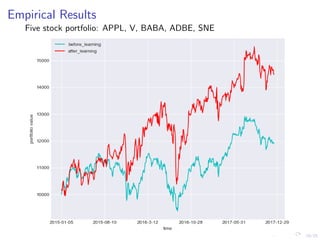
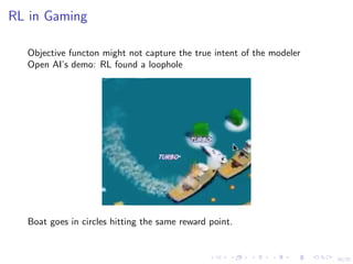
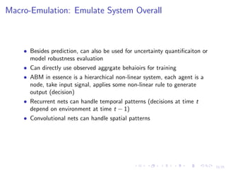
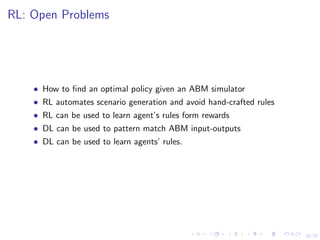
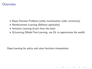
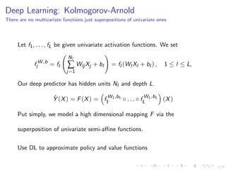
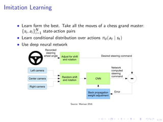
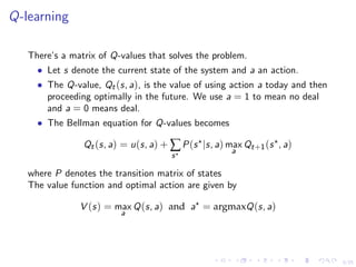
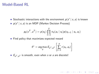
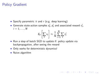
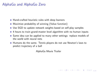
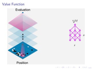
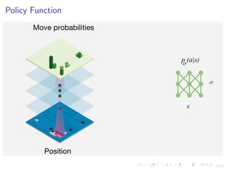
This document discusses using deep reinforcement learning and deep learning techniques for agent-based models. It discusses using deep learning to approximate policy and value functions, using imitation learning to learn from expert demonstrations, and using Q-learning and model-based reinforcement learning to optimize agent behavior. Micro-emulations use deep learning to model individual agent behavior, while macro-emulations aim to emulate the overall system behavior. Open problems include using reinforcement learning to find optimal policies given an agent-based model simulator.

1. 1/25
Deep Reinforcement Learning for Agent-Based
Models
GDRR Opening Workshop at SAMSI
Nick Polson and Vadim Sokolov
Chicago Booth and George Mason U
August 5-9, 2019

2. 2/25
Overview
• Bayes Decision Problems (utilty maximization under uncertainy)
• Reinforcement Learning (Bellman optimality)
• Imitation Learning (Learn from the best)
• Q-Learning (Model Free Learning, use DL to approximate the world)
Deep Learning for policy and value functions interpolation

3. 3/25
Deep Learning: Kolmogorov-Arnold
There are no multivariate functions just superpositions of univariate ones
Let f1, . . . , fL be given univariate activation functions. We set
f W ,b
l = fl
Nl
∑
j=1
Wlj Xj + bl = fl (Wl Xl + bl ) , 1 ≤ l ≤ L,
Our deep predictor has hidden units Nl and depth L.
ˆY (X) = F(X) = f W1,b1
1 ◦ . . . ◦ f WL,bL
L (X)
Put simply, we model a high dimensional mapping F via the
superposition of univariate semi-affine functions.
Use DL to approximate policy and value functions

4. 4/25
Imitation Learning
• Learn form the best. Take all the moves of a chess grand master:
{si , ai }N
i=1 state-action pairs
• Learn conditional distribution over actions πθ(at | st)
• Use deep neural network
the image from the nearest camera. Precise viewpoint transformation requires 3D scene knowledge
which we don’t have. We therefore approximate the transformation by assuming all points below
the horizon are on flat ground and all points above the horizon are infinitely far away. This works
fine for flat terrain but it introduces distortions for objects that stick above the ground, such as cars,
poles, trees, and buildings. Fortunately these distortions don’t pose a big problem for network train-
ing. The steering label for transformed images is adjusted to one that would steer the vehicle back
to the desired location and orientation in two seconds.
A block diagram of our training system is shown in Figure 2. Images are fed into a CNN which
then computes a proposed steering command. The proposed command is compared to the desired
command for that image and the weights of the CNN are adjusted to bring the CNN output closer to
the desired output. The weight adjustment is accomplished using back propagation as implemented
in the Torch 7 machine learning package.
Left camera
Center camera
Right camera
Random shift
and rotation
Adjust for shift
and rotation
CNN
-
Back propagation
weight adjustment
Recorded
steering
wheel angle
Network
computed
steering
command
Desired steering command
Error
Figure 2: Training the neural network.
Once trained, the network can generate steering from the video images of a single center camera.
This configuration is shown in Figure 3.
Source: Mariusz 2016

5. 5/25
Q-learning
There’s a matrix of Q-values that solves the problem.
• Let s denote the current state of the system and a an action.
• The Q-value, Qt(s, a), is the value of using action a today and then
proceeding optimally in the future. We use a = 1 to mean no deal
and a = 0 means deal.
• The Bellman equation for Q-values becomes
Qt(s, a) = u(s, a) + ∑
s
P(s |s, a) max
a
Qt+1(s , a)
where P denotes the transition matrix of states
The value function and optimal action are given by
V (s) = max
a
Q(s, a) and a = argmaxQ(s, a)

6. 6/25
Model-Based RL
• Stochastic interactions with the environment p(s | s, a) is known
• p(s | s, a) is an MDP (Markov Decision Process)
pθ(sT
, aT
) = p(s1)
T
∏
t=1
πθ(at | st)p(st+1 | st, at)
• Find policy that maximizes expected reward
θ∗
= arg max
θ
EsT ,aT
T
∑
t=1
r(st, at)
• EsT ,aT is smooth, even when s or a are discrete!

7. 7/25
Policy Gradient
• Specify parametric π and r (e.g. deep learning)
• Generate state-action samples si
t, ai
t and associated reward ri
t ,
i = 1, . . . , N
Eθ ∑
t
rt ≈
1
N
N
∑
i=1
∑
t
ri
t
• Run a step of batch SGD to update θ: policy update via
backpropagation, after seeing the reward
• Only works for deterministic dynamics!
• Naive algorithm

8. 8/25
AlphaGo and AlphaGo Zero
• Hand-crafted heuristic rules with deep learners
• Maximize probability of winning (Value function)
• Use SGD to update network weights based on self-play samples
• 4 hours to train grand-master level algorithm with no human inputs
• Same idea can be applied to many other settings: replace models of
the world with neural nets
• Humans do the same. Tennis players do not use Newton’s laws to
predict trajectory of a ball
AlphaGo Movie Trailer

9. 9/25
Value Function
Value network
Evaluation
Position
s
v (s)

10. 10/25
Policy Function Policy network
Move probabilities
Position
s
p (a|s)

11. 11/25
Full Tree
Exhaustive search

12. 12/25
Monte-Carlo rollouts
Monte-Carlo rollouts

13. 13/25
Reducing depth with value network
Reducing depth with value network
• Value function approximates probability of winning.
• Pick the path with highest approximated chance to win the game
• No need to explore the tree till the end

14. 14/25
Reducing breadth with policy network
Reducing breadth with policy network
• Policy function gives a histogram over possible moves
• Pick a few with highest probabilities
• No need to explore low probability moves, reduce breadth of the
search

15. 15/25
Deep RL for Porfolio
• Every ∆t = 30 minutes re-allocate funds
• Use vt - price vector at the end of period t
• vh
t and vl
t are high and low proces for the period t
• Relative return is yt = vt/vt−1
• pt = pt−1ytwt−1 is portfolio value at the end of period t
The goal of portfolio manager it to re-calculate weights wt → wt+1,
given Xt = (yt, yth, ytl ), yt = (yt−n+1, . . . , yt)

16. 16/25
Deep RL for Porfolio
The goal is to maximize the final portfolio return R, as a function of
states st = (Xt, wt−1) and actions at = wt
R(s1, a1, · · · , stf
, atf
, stf+1) =
1
tf
ln
pf
p0
=
1
tf
tf+1
∑
t=1
ln (µtyt wt−1) (1)
=
1
tf
tf+1
∑
t=1
rt. (2)
pf = p0 exp
tf +1
∑
t−1
rt = p0
t+1
∏
t=1
yt wt−1
‘’

17. 17/25
Policy Gradient
• Goal is to find an optimal policy πθ : S → A, here πθ is a deep
learner
• Optimize the reward
J(πθ) = R s1, πθ(s1), · · · , stf
, πθ(stf
), stf+1
• Use SGD
θ −→ θ + λ θJ[0,tf](πθ).

18. 18/25
Network Architecture
Deep Portfolio Management
portfolio vector
+1=12 elements
0.1
0.2
0.0
0.0
0.0
0.0
0.5
0.0
0.0
0.1
0.0
0.1
3 features
=11×50
price history
as input
RNN (unrolling)
20 units 50 steps
20+1 feature
maps of
size 11×1
1 features
map of
size 11×1
1×1
convolution
...
cash bias
softmax
A A A
...
from last period
Figure 3: RNN (Basic RNN or LSTM) Implementation of the EIIE: This is a recurrent
realization the Ensemble of Identical Independent Evaluators (EIIE). In this ver-
sion, the price inputs of individual assets are taken by small recurrent subnets.
These subnets are identical LSTMs or Basic RNNs. The structure of the ensem-
ble network after the recurrent subnets is the same as the second half of the CNN
in Figure 2.

19. 19/25
Empirical Results
Five stock portfolio: APPL, V, BABA, ADBE, SNE

20. 20/25
RL in Gaming
Objective functon might not capture the true intent of the modeler
Open AI’s demo: RL found a loophole
Boat goes in circles hitting the same reward point.

21. 21/25
Agent nodels are essential emitation learning
• When we design rules for individual agents we “mimic” actual
agents in real world
• It can be hand-crafted set of rules
• Statistical models, e.g. discrete choice
• A rich set of statistical learning tools is applicable by never used
• Next step: reinforcement learning for ABMs
Essentially, Herbert Simons approach described in “Sciences of the
Artificial”
We can use DL to emulate!?

22. 22/25
Micro-Emulaions for individual Agents
• Each Agent’s behavioir is modeled by a neural network
• Change multinimal logit with DL
• Instead of using survey data and past histories, use self-play
• Allows to model heterogeneity

23. 23/25
Macro-Emulation: Emulate System Overall
• Besides prediction, can also be used for uncertainty quantificaiton or
model robustness evaluation
• Can directly use observed aggrgate behaioirs for training
• ABM in essence is a hierarchical non-linear system, each agent is a
node, take input signal, applies some non-linear rule to generate
output (decision)
• Recurrent nets can handle temporal patterns (decisions at time t
depend on environment at time t − 1)
• Convolutional nets can handle spatial patterns

24. 24/25
RL: Open Problems
• How to find an optimal policy given an ABM simulator
• RL automates scenario generation and avoid hand-crafted rules
• RL can be used to learn agent’s rules form rewards
• DL can be used to pattern match ABM input-outputs
• DL can be used to learn agents’ rules.

25. 25/25
AIQ: People & Robots Smarter Together