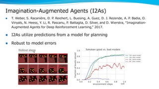
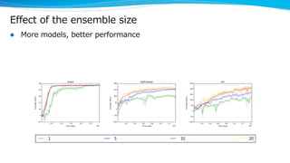
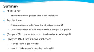
Model-based reinforcement learning techniques were presented that use learned models to improve upon model-free deep reinforcement learning. Several papers augmented deep networks with model-based components like planners or simulators to leverage predictions and reduce sample complexity. Techniques included using model rollouts to augment state representations, learning abstract state representations to simplify value prediction, and optimizing policies on ensemble models. While model-based methods show promise in addressing deep RL limitations, challenges remain in learning accurate models and developing policies robust to model errors.

1. Model-Based Reinforcement Learning
@NIPS2017
Yasuhiro Fujita
Engineer
Preferred Networks, Inc.

2. Model-Based Reinforcement Learning (MBRL)
l Model = simulator = dynamics = T(s,a,sʼ)
– may or may not include the reward function
l Model-free RL uses data from the environment only
l Model-based RL uses data from a model (which is given or estimated)
u to use less data from the environment
u to look ahead and plan
u to explore
u to guarantee safety
u to generalize to different goals

3. Why MBRL now?
l Despite deep RLʼs recent success, itʼs still difficult to see its real-world
applications
– Requiring a huge amount of interactions (1M~1000M😨)
– No safety guarantees
– Difficult to transfer to other tasks
l MBRL can be a solution for these problems
l This talk introduces some MBRL papers from the NIPS 2017 conference
and the deep RL symposium

4. Imagination-Augmented Agents (I2As)
l T. Weber, S. Racanière, D. P. Reichert, L. Buesing, A. Guez, D. J. Rezende, A. P. Badia, O.
Vinyals, N. Heess, Y. Li, R. Pascanu, P. Battaglia, D. Silver, and D. Wierstra, “Imagination-
Augmented Agents for Deep Reinforcement Learning,” 2017.
l I2As utilize predictions from a model for planning
l Robust to model errors

5. The I2A architecture (1)
l Model-free path: feed-forward net
l Model-based path:
– Make multi-step predictions (=rollouts)
from current observation and for each
action
– Encode each rollout with LSTMs
– Aggregate each code by concatenation

6. The I2A architecture (2)
l The imagination core
– consists of a rollout policy and a
pretrained environment model
– predicts next observation and
reward
l The rollout policy is distilled
online from the I2A policy

7. Value Prediction Networks
l J. Oh, S. Singh, and H. Lee, “Value Prediction Network,” in NIPS, 2017.
l Directly predicting observations in pixels might be not a good idea
– They contain irrelevant details to the agent
– They are unnecessarily high-dimensional and difficult to predict
l VPNs learn abstract states and their model by minimizing value
prediction errors

8. The VPN architecture
l x:observation o:option(≒action here)
l Decompose Q(x,o) = r(sʼ) +γV(sʼ)

9. Planning by VPNs
l The depth and width are
fixed
l Values are averaged over
prediction steps

10. Training VPNs
l V(s) of each abstract state is fit to the value from planning
l Improves performance on 2D random grid worlds and some games in
Atari, combined with Async n-step Q-learning
– surpasses observation prediction on the grid worlds

11. QMDP-net (not RL but Imitation Learning)
l P. Karkus, D. Hsu, and W. S. Lee, “QMDP-Net: Deep Learning for Planning under Partial
Observability,” in NIPS, 2017.
l A POMDP (partially observable MDP) and its solver are modeled as a
single neural network and trained end-to-end to predict expert actions
– Value Iteration Networks (NIPS 2016) were for fully observable domains

12. POMDPs and the QMDP algorithm
l In a POMDP
– The agent can only observe o ~ O(s), not s
– A belief state is considered instead: b(s) = probability of being in s
l QMDP: an approximate algorithm for solving a POMDP
1. Compute Q_{MDP}(s,a) of the underlying MDP for each (s,a) pair
2. Compute the current belief b(s) = probability of the current state being s
3. Approximate Q(b,a) ≒ Σ_s b(s)Q_{MDP}(s,a)
4. Choose argmax_a Q(b,a)
– Assumes that any uncertainty in belief will be gone after the next action

13. The QMDP-net architecture (1)
l Consists of a Bayesian filter and QMDP planner
– Bayesian filter outputs b
– QMDP planner outputs Q(b,a)

14. The QMDP-net architecture (2)
l Everything is represented as a CNN
l Works on abstract observations/states/actions that can be different from
real observations/states/actions
– abstract state = position in the plane used in CNNs

15. Performance of the QMDP-net
l Expert actions are taken from successful trajectories of the QMDP algorithm, which solves the
ground-truth POMDP
l QMDP-net surpasses normal recurrent nets and even the QMDP algorithm (because it can fail)

16. MBRL with stability guarantees
l F. Berkenkamp, M. Turchetta, A. P. Schoellig, and A. Krause, “Safe Model-based
Reinforcement Learning with Stability Guarantees,” in NIPS, 2017.
l Aims to guarantee stability (= recoverability to stable states) when there
is uncertainty in model estimation in continuous control
– Achieves both safe policy update and safe exploration
l Repeat
– Estimate the region of attraction
– Safely explore to reduce uncertainty in the model
– Update the model (e.g. Gaussian process)
– Safely improve a policy to maximize some objective

17. How it works
l Can safely optimize a neural network policy on a simulated inverted
pendulum, without the pendulum ever falling down

18. RL on a learned model
l A. Nagabandi, G. Kahn, R. S. Fearing, and S. Levine, “Neural Network Dynamics for Model-
Based Deep Reinforcement Learning with Model-Free Fine-Tuning,” 2017.
l If you can optimize a policy on a learned model, you may need less data
from the environment
– And NNs are good at prediction
l One way to learn a policy on a learned model
– Model Predictive Control (MPC)

19. Model learning is difficult
l Even small prediction errors compound and eventually diverge
– Policies learned/computed purely from simulated experiences may fail

20. Fine-tuning a policy with model-free RL
l Outperforms pure model-free RL by
1. Collect data, fit a model and apply MPC
2. Train a NN policy to imitate actions of MPC
3. Fine-tune the policy with model-free RL (TRPO)

21. Model ensemble
l T. Kurutach and A. Tamar, “Model-Ensemble Trust-Region Policy Optimization,” in NIPS Deep
Reinforcement Learning Symposium, 2017.
l Another way to learn a policy on a learned model
– Apply model-free RL on a learned model
l Model-Ensemble Trust Region Policy Optimization (ME-TRPO)
1. Fit an ensemble of NN models to predict next states
u Why ensemble? To maintain model uncertainty
2. Optimize a policy on simulated experiences with TRPO until performance
stops to increase
3. Collect new data for model learning and go to 1

22. Effect on sample-complexity
l Improves sample complexity on MuJoCo-based continuous control tasks
– x-axis is time steps in a log scale

23. Effect of the ensemble size
l More models, better performance

24. Summary
l MBRL is hot
– There were more papers than I can introduce
l Popular ideas
– Incorporating a model/planning structure into a NN
– Use model-based simulations to reduce sample complexity
l (Deep) MBRL can be a solution to drawbacks of deep RL
l However, MBRL has its own challenges
– How to learn a good model
– How to make use of a possibly bad model