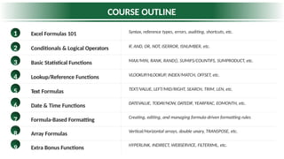
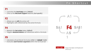
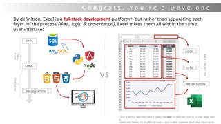
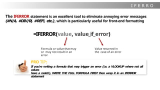
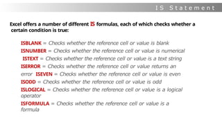
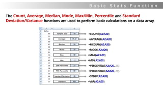
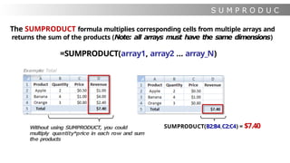
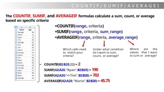
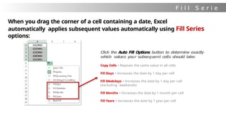
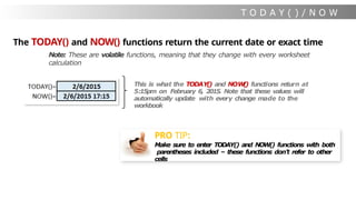
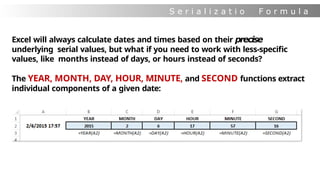
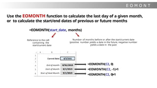
The document outlines a comprehensive course on Microsoft Excel formulas and functions, covering essential topics such as syntax, logical operators, statistical functions, lookup/reference functions, and more. It emphasizes the use of Excel's formula library, various auditing tools, and keyboard shortcuts to enhance efficiency. Additionally, it provides insight into conditional statements, data validation, and error handling techniques to facilitate effective spreadsheet management.

1. MICROSOFT EXCEL:
FORMULAS &
FUNCTIONS

2. COURSE OUTLINE
1 Excel Formulas 101 Syntax, reference types, errors, auditing, shortcuts, etc.
2 Conditionals & Logical Operators IF, AND, OR, NOT, ISERROR, ISNUMBER, etc.
3 Basic Statistical Functions MAX/MIN, RANK, RAND(), SUMIFS/COUNTIFS, SUMPRODUCT, etc.
4 Lookup/Reference Functions VLOOKUP/HLOOKUP, INDEX/MATCH, OFFSET, etc.
5 Text Formulas TEXT/VALUE, LEFT/MID/RIGHT, SEARCH, TRIM, LEN, etc.
6 Date & Time Functions DATEVALUE, TODAY/NOW, DATEDIF, YEARFRAC, EOMONTH, etc.
7 Formula-Based Formatting Creating, editing, and managing formula-driven formatting rules
8 Array Formulas Vertical/Horizontal arrays, double unary, TRANSPOSE, etc.
9 Extra Bonus Functions HYPERLINK, INDIRECT, WEBSERVICE, FILTERXML, etc.

3. SETTING EXPECTATIONS
1 We’ll be using Excel for Windows/PC (Excel 2013-2019)
• What you see on your screen will not always match mine, especially if you’re using an older version of Excel
We’ll focus on many of Excel’s most powerful, widely-used functions
2
The goal of this course is to help you master the building blocks
3
• Excel’s formula library includes nearly 500 functions; we won’t cover some of the more specialized categories
(like Financial or Engineering functions), or those which require knowledge outside the scope of this course
• The beauty of Excel formulas is that no matter how complex they get, they’re ALL comprised of simple pieces.
We’ll start by mastering each individual component before combining them in more complex ways
Feeling stuck? We’ve got your back.
4
• If you have questions about the course material, feel free to post a question and we’ll be happy to help
• For project-specific questions, recommend posting to the answers.microsoft.com community forum

4. FORMULAS 101

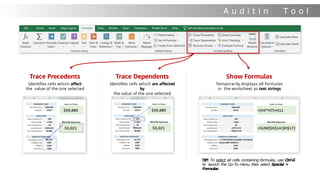
5. F o r m u l a S y n t a
x
= MATCH(lookup_value, lookup_array,
[match_type])
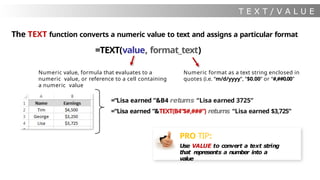
The function name tells Excel what
type of operation you’re about to
perform (Excel offers ~500
functions)
Note: Function names aren’t case-
sensitive, and aren’t always
required; basic arithmetic and
logical operations often don’t need
one:
• = A1 + B1
• = A1 /
B1
• = A1 >
B1
• = A1 =
B1
These are arguments, which vary by function and
provide
Excel with the info needed to evaluate a result
Note: Not all arguments are required; optional
arguments are surrounded by square brackets (like
[match_type] above)
Most functions have at least one required argument, but
some
don’t require any, like ROW(), COLUMN(), TODAY() or NOW()
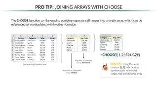
PRO TIP:
As you begin writing a formula, the Function ScreenTips box will
guide you through each individual argument – this is an extremely
helpful tool!
All formulas start
with an equals sign
Arguments are always
surrounded by
parentheses
Arguments are separated by commas in the US, but
other regions may use different list separators (like
semi-colons)

6. R e f e r e n c e T y p e
s
Fixed Column &
Row
Relative Column, Fixed
Row
Fixed Column, Relative
Row
Relative Column &
Row
PRO TIP:
Mastering reference types is my #
1
tip
for working efficiently with formulas
Reference types allow you to “recycle” formulas across multiple cells, without
having to manually update your references (which would be completely
impractical)
Cell references are relative by default (A1).
This allows the reference to change as the
formula is copied to new cells
The $ symbol is used to create fixed
references. You can fix entire cells ($A$1) or just
the column ($A1) or row (A$1), which prevents
references from changing as the formula is
copied to new cells

7. C o m m o n E r r o r
s
Error Type What it means
Column isn’t wide enough to display values
How to fix it
Excel does not recognize text in a formula
Formula has the wrong type of
argument
Formula is dividing by zero or an empty cell
Formula refers to a cell that is not
valid
Formula can’t find a referenced
value
Drag or double-click column border to increase width, or right-
click to set custom column width
Make sure that function names are correct, references are valid
and spelled properly, and quotation marks and colons are in
place
Check that your formula isn’t trying to perform an arithmetic
operation on text strings or cells formatted as text
Check the value of your divisor; if 0 is correct, use an IF
statement to display an alternate value if you choose
Make sure that you didn’t move, delete, or replace cells that
are
referenced in your formula
Check that all references and formula arguments evaluate
properly (the most common cause is a lookup value with no
match)
#
#
#
#
#
#
#NAME?
#VALUE!
#DIV/0!
#REF!
#N/A

8. A u d i t i n
g
T o o l
s
Trace Precedents
Identifies cells which affect
the value of the one selected
Trace Dependents
Identifies cells which are affected
by
the value of the one selected
Show Formulas
Temporarily displays all formulas
in the worksheet as text strings
TIP: To select all cells containing formulas, use Ctrl-G
to launch the Go-To menu, then select Special >
Formulas

9. A u d i t i n
g
T o o l
s
1 2 3 4 5 6
Evaluate Formula
Allows you to cycle through
each individual calculation step
within a formula, see how each
component evaluates, and
pinpoint the source of the error
PRO TIP:
Evaluate Formula is my go-to tool for breaking down complex or unfamiliar formulas

10. A u d i t i n
g
T o o l
s
Error Checking
Scans the sheet for errors and
provides a summary with
options to trace the source,
ignore the error, modify your
options, or link out to
Microsoft support

11. Ctrl + Arrow
• Jumps to the last cell in a data region, in the direction of the
arrow
C T R L S h o r t c u t
s
Ctrl + Home/End
• Jumps to the Home (top-left) or End (bottom-right) cell in a region
https://exceljet.net/keyboard-
shortcuts
FULL LIST:
Ctrl + Shift + Arrow
• Selects to the last cell in a data region, in the direction of the
arrow
Ctrl + .
• Jumps straight to each corner within a selected cell range
Ctrl + PgUp/PgDn
• Switches worksheet tabs, either to the left (PgUp) or right (PgDn)
Ctrl + Shift
+
Ctrl + Shift
+
Ctrl + Shift +
End

12. F n S h o r t c u t
s
F1
• Launches the Excel help pane (default)
• Links to the Microsoft Support website (tool-specific)
F2
• Allows you to edit the active cell
• Highlights cells referenced by the active formula
F4
• Repeats the last action taken (default)
• Toggles absolute/relative cell references within a formula
F9
• Calculates all workbook formulas (when in manual mode)
• Evaluates each function argument within the formula bar
A1
A$
1
$A1 F4 $A$1
https://exceljet.net/keyboard-
shortcuts
FULL LIST:

13. Mac Shortcut Purpose PC Equivalent
Command-T Cycles between cell reference types F4
Command-Y Repeats the last user action F4
Control-U Displays cell ranges tied to a given formula F2
C o m m o n M a c S h o r t c u t
s
Jumps to the edge of a contiguous data
array
Command-Shift-Arrow E
xt
e
n
ds a s
elec
tion to t
h
e e
d
g
e of a d
a
t
a a
r
r
a
y CTRL-SHIFT-ARROW
Jumps between workbook
tabs
Command-Arrow CTRL-ARROW
CTRL-PAGE UP/DOWN
https://exceljet.net/keyboard-
shortcuts
FULL LIST:
Command-Fn-Up/Down

14. A l t K e y T i p
s
Alt Key Tips
• Allow you to quickly access tools from ribbon menus
and sub-menus using only the keyboard (no clicks!)
• Each keystroke takes you a layer deeper, until you land
on the tool you need (Note: Simply press & release the
Alt key, instead of holding it down)
• There are hundreds of combinations, so start by
focusing on the tools that you use most frequently:
Alt – H – V – V
• Paste Special as Values
Alt – A – T
• Add or remove filters
Alt – M – V
• Evaluate Formula
Some of
my go-to
key tips

15. D a t
a
V a l i d a t i o
n
Data Validation
Restricts the values that a user can enter into a given
cell, based on:
• Number Type (Whole vs. Decimal)
• Value (Between, Less Than, Equal To, etc)
• List of Items (Based on cell range or manual
list)
• Date/Time (Between, Less Than, Equal To, etc)
• Text Length (Between, Less Than, Equal To,
etc)
• Custom (Formula-Driven)
FUN FACT: You can customize your own error
alerts!
Decimal from 0
-1
List of
Items

16. C o n g r a t s , Y o u ’ r e a D e v e l o p e
r !
DATA
LOGIC
PRESENTATION
LOGIC
DATA
BACK-
END
FRONT-END
By definition, Excel is a full-stack development platform*; but rather than separating each
layer of the process (data, logic & presentation), Excel mixes them all within the same
user interface:
BACK
+
FRONT
END
PRESENTATION
VS
*This is NOT a claim that Excel is always the right full-stack dev tool (or, in may cases, even
a
viable one). Rather, it’s an effort to inspire users to think creatively about what Excel can do

17. CONDITIONAL STATEMENTS

18. C o n d i t i o n a
l
S t a t e m e n t
s
All Conditional Statements in Excel are
based on simple “IF/THEN” statements:
-I
F it’s raining, THEN bring an umbrella
-I
F it’s sunny, THEN bring sunglasses
-IF it’s sunny AND it’s summer, skip work and go to the
beach
You’re basically saying “Hey Excel, if this statement
is true, do this. Otherwise, do something else.”

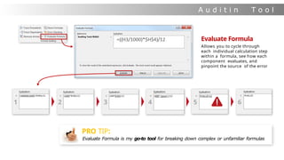
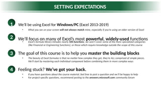
19. I F
S t a t e m e n t s
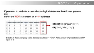
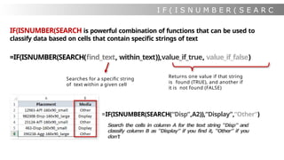
=IF(logical_test, [Value if True], [Value if False])
Any test that results in
either
TRUE or FALSE
(i.e. A1=“Google”, B2<100,
etc)
Value returned if
logical test is TRUE
Value returned if
logical test is FALSE
= IF(B2<=0,“Yes”,”No”)
I
n this case we’re categorizing the Freeze
column as “Yes” if the temperature is equal
to or below 32, otherwise “No”

20. N e s t e d I F S t a t e m e n t
s
= IF(B2<40,”COLD”,IF(B2>80,”HOT”,”MILD”))
If temp<40, climate = “Cold”, if
temp>80, climate = “Hot”, otherwise
climate = “Mild”
By using Nested IF Statements, you can include multiple logical
tests within a single formula:

21. A N D / O R S t a t e m e n t
s
Excel’s AND and OR statements allow you to include multiple logical tests at once:
=IF(OR(F2=“Rain”,F2=“Snow”),“Wet",“Dry")
Here we’re categorizing conditions as “Wet”
if the precipitation type equals “rain” OR
“snow”, otherwise Conditions = “Dry”
=IF(AND(D2=“Yes”,C2>0),“Snow",IF(AND(D2=“No”,C2>0),“Rain",“None"))
If the temp is below freezing AND the amount of precipitation > 0, then Precip Type = “Snow”, if
the temp is
above freezing AND the amount of precipitation >0, then Precip Type = “Rain”, otherwise Precip
Type = “None”
PRO TIP:
When writing nested functions, copy/paste repetitivepieces and
tweak individual elements to save time (rather than starting from
scratch)

22. N O T / <
>
O p e r a t o r
s
I
n both of these examples, we’re defining Conditions = “Wet” if the amount of precipitation is NOT
equal to 0
If you want to evaluate a case where a logical statement is not true, you can
use
either the NOT statement or a “<
>” operator
=IF(NOT(C2=0),“Wet",“Dry")
=IF(C2<>0,“Wet",“Dry")

23. I F E R R O
R
Formula or value that may
or may not result in an
error
The IFERROR statement is an excellent tool to eliminate annoying error messages
(#N/A, #DIV/0!, #REF!, etc.), which is particularly useful for front-end formatting
=IFERROR(value, value_if_error)
Value returned in
the case of an error
PRO TIP:
If you’re writing a formula that may trigger an error (i.e. a VLOOKUP where not all
values
have a match), WRITE THE FULL FORMULA FIRST then wrap it in an IFERROR
statement

24. I S S t a t e m e n t
s
Excel offers a number of different IS formulas, each of which checks whether a
certain condition is true:
ISBLANK = Checks whether the reference cell or value is blank
ISNUMBER = Checks whether the reference cell or value is numerical
ISTEXT = Checks whether the reference cell or value is a text string
ISERROR = Checks whether the reference cell or value returns an
error ISEVEN = Checks whether the reference cell or value is even
ISODD = Checks whether the reference cell or value is odd
ISLOGICAL = Checks whether the reference cell or value is a logical
operator
ISFORMULA = Checks whether the reference cell or value is a
formula

25. COMMON STATS FUNCTIONS

26. B a s i c S t a t s F u n c t i o n
s
The Count, Average, Median, Mode, Max/Min, Percentile and Standard
Deviation/Variance functions are used to perform basic calculations on a data array
=COUNT(A2:A20)
=AVERAGE(A2:A20)
=MEDIAN(A2:A20)
=MODE(A2:A20)
=MAX(A2:A20)
=MIN(A2:A20)
=PERCENTILE(A2:A20,.25)
=PERCENTILE(A2:A20,.75)
=STDEV(A2:A20)
=VAR(A2:A20)

27. R A N K / S M A L L / L A R G
E
The RANK function returns the rank of a
particular number among a list of
values
RANK(A2,A2:A8) = 2
RANK(A3,A2:A8) = 7 (lowest)
RANK(A4,A2:A8) = 6
RANK(A5,A2:A8) = 1 (highest)
RANK(A6,A2:A8) = 4
RANK(A7,A2:A8) = 3
RANK(A8,A2:A8) = 5
The SMALL/LARGE functions return the
nth smallest/largest values within an array
SMALL(A2:A8,3) = 50
(the 3rd smallest number in the array is
5
0)
LARGE(A2:A8,2) = 90
(the 2nd largest number in the array
is 90
)

28. P E R C E N T R A N
K
PERCENTRANK returns the rank of a value as
a percentage of a given array or dataset
=PERCENTRANK(array, x)
What range of
data are you
looking at?
Which value within the
range are you looking
at?
PERCENTRANK($A$2:$A$19, A14) = 100% (highest)
PERCENTRANK($A$2:$A$19, A16) = 0% (lowest)

29. R A N D / R A N D B E T W E E
N
RAND() and RANDBETWEEN act like random number generators in Excel:
The RAND() function returns a random
value between 0 and 1 (to 15 digits)
The RANDBETWEEN function returns an
integer between two values that you specify
=RANDBETWEEN(0,100
)

30. S U M P R O D U C
T
The SUMPRODUCT formula multiplies corresponding cells from multiple arrays and
returns the sum of the products (Note: all arrays must have the same dimensions)
=SUMPRODUCT(array1, array2 … array_N)
SUMPRODUCT(B2:B4,C2:C4) = $7.40
Without using SUMPRODUCT, you could
multiply quantity*price in each row and sum
the products
Example: Total
Revenue

31. S U M P R O D U C
T
SUMPRODUCT is often used with filters to calculate products only for rows that
meet certain criteria:
Quantity of goods sold at Shaws:
SUMPRODUCT((A2:A17=“Shaws”)*C2:C17) = 16
Total revenue from Shaws:
SUMPRODUCT((A2:A17=“Shaws”)*C2:C17*D2:D17) = $21.80
Revenue from apples sold at Shaws:
SUMPRODUCT((A2:A17=“Shaws”)*(B2:B17=“Apple”)*C2:C17*D2:D17) =
$0.50
PRO TIP:
When you add filters to a SUMPRODUCT, you
need to change the commas to multiplication
signs

32. S U M P R O D U C
T
Great, but how does it really work?
SUMPRODUCT((A2:A17=“Shaws”)*(B2:B17=“Apple”)*C2:C17*D2:D17) = $0.50
What YOU see
What EXCEL sees
When you apply a condition or
filter to a column, Excel
translates those cells as 0’s (if
false) and 1’s (if true)
If you multiply all four
columns, ONLY ROWS
THAT SATISFY ALL
CONDITIONS WILL
PRODUCE A NON-ZERO
SUM

33. C O U N T I F / S U M I F / A V E R A G E I
F
Which cells need
to match your
criteria?
Under what condition
do I want to sum,
count, or average?
Where are the
values that I want
to sum or average?
The COUNTIF, SUMIF, and AVERAGEIF formulas calculate a sum, count, or average
based on specific criteria
=COUNTIF(range, criteria)
=SUMIF(range, criteria, sum_range)
=AVERAGEIF(range, criteria, average_range)
COUNTIF(B2:B20,22) = 2
SUMIF(A2:A20,“Ryan”,B2:B20) = 190
SUMIF(A2:A20,“<>Tim”,B2:B20) = 702
AVERAGEIF(A2:A20,“Maria”,B2:B20) = 45.75

34. C O U N T I F S / S U M I F S / A V E R A G E I F S
COUNTIFS, SUMIFS, and AVERAGEIFS are used when you want to evaluate a
count, sum, or average based on multiple conditions or criteria
=COUNTIFS(criteria_range1, criteria1, criteria_range2 , criteria2…)
=SUMIFS(sum_range, criteria_range1, criteria1, criteria_range2 , criteria2…)
=AVERAGEIFS(average_range, criteria_range1, criteria1, criteria_range2 , criteria2…)
COUNTIFS(B2:B13,“Search”, D2:D13,“>200”) = 3
SUMIFS(D2:D13, A2:A13,“Feb”,B2:B13,“Display”) = 734
AVERAGEIFS(D2:D13, A2:A13,“Jan”,C2:C13,“MSN”) = 263
PRO TIP:
If you use < or >
, you need to add
quotation
marks as you would with text (i.e.
“>200”)

35. LOOKUP & REFERENCE FUNCTIONS

36. N a m e
d
R a n g e
s
Using Named Arrays can simplify a lookup function if you use the
same
data array in multiple formulas
For example, if you name the array from A1:D6
“Apparel”…
…you can write your vlookup formula in
either of
the following ways:
=VLOOKUP(A1,$A$1:$D$6,2)
=VLOOKUP(A1,Apparel,2)

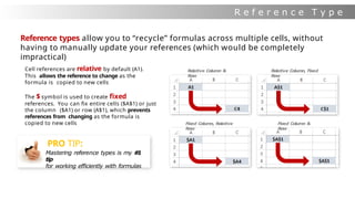
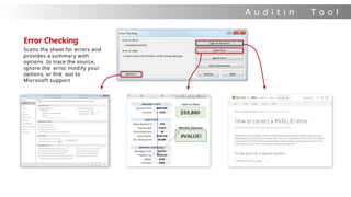
37. V L O O K U
P
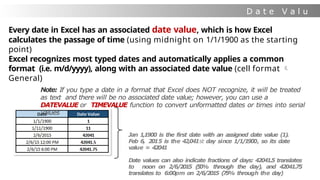
Let’s take a look at one of Excel’s most common reference functions – VLOOKUP:
=VLOOKUP(lookup_value, table_array, col_index_num, [range_lookup])
This is the value that
you are trying to
match in the table
array
This is where you
are looking for
the lookup value
Which column
contains the data
you’re looking
for?
Are you trying to match
the exact lookup value (0),
or something similar (1)?
D2=VLOOKUP(A2, $G$1:$H$5, 2, 0)
To populate the Price in
column D, we look up the
name of the product in
the data array from
G1:H5 and return the
value from the 2nd column
over

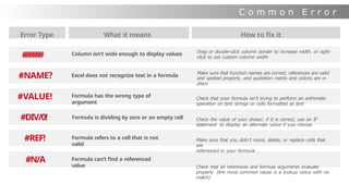
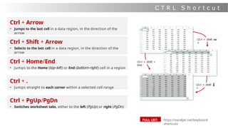
38. H L O O K U
P
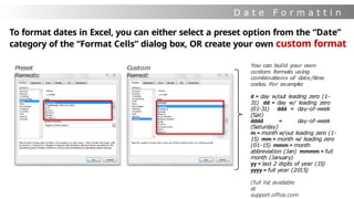
Use HLOOKUP if your table array is transposed (variables headers listed in rows)
=HLOOKUP(lookup_value, table_array, row_index_num, [range_lookup])
This is the value that
you are trying to
match in the table
array
This is where you
are looking for
the lookup value
Which row
contains the data
you’re looking
for?
Are you trying to match
the exact lookup value (0),
or something similar (1)?
D2=HLOOKUP(A2, $H$1:$L$2, 2, 0)
With an HLOOKUP, we search for the product
name in F1:J2 and return the value from the
2nd row down

39. L a w s o f L o o k u p
s
There are two key rules that constrain VLOOKUP and HLOOKUP formulas:
1. The lookup value must be in the first column of a
VLOOKUP table array or the first row of a
HLOOKUP table array
2. Excel will always return the value from the top most
row or left most column of a table array when
multiple instances of the lookup value are present
PRO TIP:
Avoid breaking Law #
2 by identifying a
“Key” that is common to both datasets
and is unique for every row (NOTE: Keys
often take the form of a concatenation of
multiple fields)

40. R O W / R O W
S
The ROW function returns the row number of a given reference, while the ROWS
function returns the number of rows in a given array or array formula
=ROW([reference])
=ROWS(array)
This example uses an array, which is
why it includes the fancy { } signs –
more on that in the ARRAY functions
section
ROW(C10) = 10
ROWS(A10:D15) = 6
ROWS({1,2,3;4,5,6}) = 2

41. C O L U M N / C O L U M N
S
The COLUMN function returns the column number of a given reference, while the
COLUMNS function returns the number of columns in a given array or array
formula
=COLUMN([reference])
=COLUMNS(array)
COLUMN(C10) = 3
COLUMNS(A10:D15) = 4
COLUMNS({1,2,3;4,5,6}) = 3
PRO TIP:
Leave the cell reference out and
just write ROW() or COLUMN(
) to
return the row or column number
of the cell in which the formula is
written

42. I N D E X
The INDEX function returns the value of a specific cell within an array
=INDEX(array, row_num, column_num)
INDEX($A$1:$C$5, 5, 3) = 234
I
n this case we’re telling Excel to find the value of a
cell somewhere within the array of A1:C5. Starting
from the upper left, we move down to the 5t
h row
and right to the 3rd column, to return the value of
234
What range of
cells are you
looking at?
How many rows
down is the
value you want?
How many
columns over is
the value you
want?

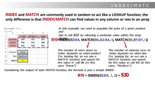
43. M A T C H
The MATCH function returns the position of a specific value within a column or row
=MATCH(lookup_value, lookup_array, [match_type])
Matching the word “Pliers” in column A,
we find it in the 4t
h row. Matching the
number 66 in row 3, we find it in the
3rd column
What value are
you trying to find
the position of?
In which row or column
are you looking? (must
be a 1-dimensional array)
Are you looking for the
exact value (0), or anything
close?
1: Find largest value < or =
lookup_value
0: Find exact lookup_value
-1: Find smallest value > or
= lookup_value
MATCH(“Pliers”,$A$1:$A$5, 0) = 4
MATCH(66,$A$3:$C$3, 0) = 3

44. I N D E X / M A T C
H
INDEX and MATCH are commonly used in tandem to act like a LOOKUP function; the
only difference is that INDEX/MATCH can find values in any column or row in an array
I
n this example, we want to populate the price of a given product
and
size in cell B10 by returning a particular value within the array
B2:D4
B10=INDEX(B2:D4, MATCH(B6,A2:A4,0), MATCH(B8,B1:D1,0))
Example: Price
Checker
The number of rows down to
index depends on what product
I’m looking for, so we use a
MATCH function and search for
the value in cell B6 (in this
case “Pants”)
The number of columns over to
index depends on what size
I’m looking for, so we use a
MATCH function and search
for the value in cell B8 (in this
case, “Medium”)
Considering the output of each MATCH function, the formula is just a simple INDEX:
B10 = INDEX(B2:D4, 3, 2) = $30

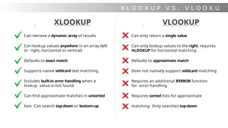
45. X L O O K U
P
XLOOKUP can retrieve values from a table or range by matching a lookup value,
and offers more flexibility than VLOOKUP, HLOOKUP, or INDEX & MATCH formulas
=XLOOKUP(lookup_value, lookup_array, return_array, [if_not_found], [match_mode], [search_mode])
Which value are
you looking to
match?
Where are you
trying to find a
match for your
lookup value?
What if the
lookup value isn’t
found in the
lookup array?
Are you looking for
an exact,
approximate, or
wildcard match?
Where are the
values
you want to
retrieve?
Do you want to
search top
down or
bottom up?
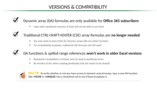
IMPORTANT NOTE: XLOOKUP is currently only available for Office 365 subscribers

46. X L O O K U P V S . V L O O K U
P
XLOOKUP
Can retrieve a dynamic array of results
Can lookup values anywhere in an array (left
or right, horizontal or vertical)
Defaults to exact match
Supports native wildcard text matching
Includes built-in error handling when a
lookup value is not found
Can find approximate matches in unsorted
lists Can search top-down or bottom-up
VLOOKUP
Can only return a single value
Can only lookup values to the right, requires
HLOOKUP for horizontal matching
Defaults to approximate match
Does not natively support wildcard matching
Requires an additional IFERROR function
for error handling
Requires sorted lists for approximate
matching Only searches top-down

47. C H O O S
E
The CHOOSE function selects a value, cell reference, or function to perform from
a list, based on a given index number
=CHOOSE(index_num, value1, [value2], …)
Which item in the
following list should be
evaluated?
1st item
in the
list
2nd item
in the
list
3rd, 4th, 5th, etc…
FUN FACTS ABOUT CHOOSE:
• List items can include numbers, cell references, defined names, formulas, or text (or a mix!)
• CHOOSE acts like an INDIRECT function, and can interpret cell references instead of treating them
as text
• You can combine CHOOSE with other functions, or nest it directly into a cell reference

48. O F F S E
T
The OFFSET function is similar to INDEX, but can return either the value of a cell
within an array (like INDEX) or a specific range of cells
=OFFSET(reference, rows, columns, [height], [width])
What’s
your
starting
point?
How
many
rows
down
should
you
move?
How many
columns
over should
you move?
If you want to return a
multidimensional array,
how tall and wide should
it be?
An OFFSET formula where [height]=1
and [width]=1 will operate exactly like an
INDEX. A more common use of OFFSET
is to create dynamic arrays (like the
Scroll Chart example in the appendix)
PRO TIP:
Don’t use OFFSET or INDEX/MATCH when
a simple VLOOKUP will do the trick

49. TEXT FUNCTIONS

50. T R I M / U P P E R / L O W E R / P R O P E
R
Text functions can be used to standardize formatting, particularly the TRIM, UPPER,
LOWER, and PROPER functions:
PRO TIP:
If two text strings are identical except one has a trailing space, they will look exactly
the same but Excel will treat them as completely different values; TRIM will make them
equivalent

51. C O N C A T E N A T
E
CONCATENATE allows you to combine text, cell values, or formula outputs into a
single text string
Note: Rather than typing “=CONCATENATE(Text1, Text2…)”, you can
simply
separate each piece of the resulting text string with an ampersand
(“&”)

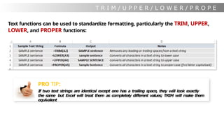
52. L E F T / M I D / R I G H T / L E
N
The LEFT, MID, and RIGHT functions return a specific number of characters from a
location within a text string, and LEN returns the total number of characters
=LEFT(text, [num_chars])
=RIGHT(text, [num_chars])
=MID(text, start_num, num_chars)

53. T E X T / V A L U E
The TEXT function converts a numeric value to text and assigns a particular format
=TEXT(value, format_text)
Numeric value, formula that evaluates to a
numeric value, or reference to a cell containing
a numeric value
Numeric format as a text string enclosed in
quotes (i.e. “m/d/yyyy”, “$0.00” or “#,##0.00”
=“Lisa earned ”&B4 returns “Lisa earned 3725”
=“Lisa earned ”&TEXT(B4“$#,###”) returns “Lisa earned $3,725”
PRO TIP:
Use VALUE to convert a text string
that represents a number into a
value

54. S E A R C H / F I N
D
The SEARCH function returns the number of the character at which a specific
character or text string is first found (otherwise returns #VALUE! error)
=SEARCH(find_text, within_text, [start_num])
What character or
string are you
searching for?
Where is the text
that you’re
searching through?
Search from the beginning
(default) or after a certain
number of characters?
PRO TIP:
The FIND function works exactly the same way, but is case-
sensitive

55. I F ( I S N U M B E R ( S E A R C
H
IF(ISNUMBER(SEARCH is powerful combination of functions that can be used to
classify data based on cells that contain specific strings of text
=IF(ISNUMBER(SEARCH(find_text, within_text)),value_if_true, value_if_false)
Searches for a specific string
of text within a given cell
Returns one value if that string
is found (TRUE), and another if
it is not found (FALSE)
=IF(ISNUMBER(SEARCH(“Disp”,A2)),”Display”,”Other”)
Search the cells in column A for the text string “Disp” and
classify column B as “Display” if you find it, “Other” if you
don’t

56. DATE & TIME FUNCTIONS

57. D a t e V a l u
e
Every date in Excel has an associated date value, which is how Excel
calculates the passage of time (using midnight on 1/1/1900 as the starting
point)
Excel recognizes most typed dates and automatically applies a common
format (i.e. m/d/yyyy), along with an associated date value (cell format 
General)
Note: If you type a date in a format that Excel does NOT recognize, it will be treated
as text and there will be no associated date value; however, you can use a
DATEVALUE or TIMEVALUE function to convert unformatted dates or times into serial
values
Jan 1,1900 is the first date with an assigned date value (1).
Feb 6, 2015 is the 42,041st day since 1
/
1
/
1
90
0, so its date
value = 42041
Date values can also indicate fractions of days: 42041.5 translates
to noon on 2
/
6
/
2
01
5 (
5
0
% through the day), and 42041.75
translates to 6:00pm on 2
/
6
/
2
01
5 (
7
5
% through the day)

58. D a t e F o r m a t t i n
g
To format dates in Excel, you can either select a preset option from the “Date”
category of the “Format Cells” dialog box, OR create your own custom format
Preset
Formats:
Custom
Format:
You can build your own
custom formats using
combinations of date/time
codes. For example:
d = day w/out leading zero (1-
31) dd = day w/ leading zero
(01-31) ddd = day-of-week
(Sat)
dddd = day-of-week
(Saturday)
m = month w/out leading zero (1-
15) mm = month w/ leading zero
(01-15) mmm = month
abbreviation (Jan) mmmm = full
month (January)
yy = last 2 digits of year (15)
yyyy = full year (2015)
(full list available
at
support.office.com

59. F i l l S e r i e
s
When you drag the corner of a cell containing a date, Excel
automatically applies subsequent values automatically using Fill Series
options:
Click the Auto Fill Options button to determine exactly
which values your subsequent cells should take:
Copy Cells = Repeats the same value in all cells
Fill Days = Increases the date by 1 day per cell
Fill Weekdays = Increases the date by 1 day per cell
(excluding weekends)
Fill Months = Increases the date by 1 month per cell
Fill Years = Increases the date by 1 year per cell

60. T O D A Y ( ) / N O W
( )
The TODAY() and NOW() functions return the current date or exact time
Note: These are volatile functions, meaning that they change with every worksheet
calculation
PRO TIP:
Make sure to enter TODAY() and NOW() functions with both
parentheses included – these functions don’t refer to other
cells
This is what the TODAY() and NOW
(
) functions return at
5:15pm on February 6, 2015. Note that these values will
automatically update with every change made to the
workbook

61. S e r i a l i z a t i o
n
F o r m u l a
s
Excel will always calculate dates and times based on their precise
underlying serial values, but what if you need to work with less-specific
values, like months instead of days, or hours instead of seconds?
The YEAR, MONTH, DAY, HOUR, MINUTE, and SECOND functions extract
individual components of a given date:

62. E O M O N T
H
Use the EOMONTH function to calculate the last day of a given month,
or to calculate the start/end dates of previous or future months
=EOMONTH(start_date, months)
Reference to the cell
containing the
start/current date
Number of months before or after the start/current date
(positive number yields a date in the future, negative number
yields a date in the past
=EOMONTH(C2, 0)
=EOMONTH(C2, -1)+1
=EOMONTH(C2, 0)+1

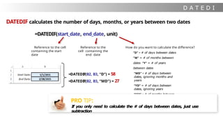
63. Y E A R F R A
C
YEARFRAC calculates the fraction of a year represented by the number of whole days
between two dates
=YEARFRAC(start_date, end_date, [basis])
Reference to the cell
containing the start
date
Reference to the
cell containing the
end date
Option specify the type of day count to
use:
0 (default) = US (NASD) 30/360
1 = actual/actual
(RECOMMENDED)
2 = actual/360
3 = actual/365
4 = European 30/360
=YEARFRAC(B2, B3, 1) = 15.9%
=YEARFRAC(B2, B3, 2) = 16.1%
PRO TIP:
YEARFRAC is a
great tool for pacing
and projection
calculations

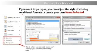
64. W E E K D A
Y
If you want to know which day of the week a given date falls on, there are
two ways to do it:
1) Use a custom cell format of either “ddd” (Sat) or “dddd” (Saturday)
-Note that this doesn’t change the underlying value, only how that value is
displayed
2)Use the WEEKDAY function to return a serial value corresponding
to a particular day of the week (either 1-7 or 0-6)
=WEEKDAY(serial_number, [return type])
This refers to a cell
containing a date or
time
0 (default) = Sunday (1) to Saturday
(7)
1 = Monday (1) to Sunday (7)
3 = Monday (0) to Sunday (6)

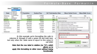
65. W O R K D A Y / N E T W O R K D A Y
S
WORKDAY returns a date that is a specified number of days before or after a given
start date, excluding weekends and (optionally) holidays; NETWORKDAYS counts the
number of workdays between two dates:
=WORKDAY(start_date, days, [holidays])
This refers to the cell
containing the start
date
Number of days
before or after
start date
Optional reference
to a list of holiday
dates
=NETWORKDAYS(start_date, end_date, [holidays])
This refers to the cell
containing the start
date
This refers to the cell Optional
reference containing the end date
to a list of holiday
dates
=WORKDAY(B2, 20) = 1/29/2015
=NETWORKDAYS(B2, B3) = 42

66. D A T E D I
F
DATEDIF calculates the number of days, months, or years between two dates
=DATEDIF(start_date, end_date, unit)
Reference to the cell
containing the start
date
Reference to the
cell containing the
end date
How do you want to calculate the difference?
“D” = # of days between dates
“M” = # of months between
dates “Y” = # of years
between dates
“MD” = # of days between
dates, ignoring months and
years
“YD” = # of days between
dates, ignoring years
“YM” = # of months between
dates, ignoring days and years
=DATEDIF(B2, B3, “D”) = 58
=DATEDIF(B2, B3, “MD”) = 27
PRO TIP:
If you only need to calculate the # of days between dates, just use
subtraction

67. FORMULA-BASED FORMATS

68. F o r m u l a - B a s e d
F o r m a t t i n g
If you want to go rogue, you can adjust the style of existing
conditional formats or create your own formula-based
rules
This is where you can add, clear, and
manage your conditional formatting
rules

69. F o r m u l a - B a s e
d
F o r m a t t i n
g
I
n this example we’re formatting the cells in
columns B through H with a green fill and bold text,
but only when the state name is equal to the value in
cell $C$2
Note that the row label is relative (no “$”), which
allows us to
apply this formatting to other rows without losing
functionality

70. DYNAMIC ARRAY FORMULAS

71. In this section we’ll introduce dynamic arrays, explore how array calculations work, and apply
powerful functions like FILTER, SORT, and UNIQUE to explore and analyze data in Excel
GOALS FOR THIS SECTION:
• Understand how dynamic array calculations and spill
ranges work
• Apply powerful array functions like FILTER, SORT,
SEQUENCE and UNIQUE
• Learn how dynamic calculations can be applied to
“legacy” functions in Excel
• Analyze data by combining dynamic array functions
DYNAMIC ARRAYS
TOPICS WE’LL COVER:
Dynamic Excel Spill Ranges
SORT & SORTBY FILTER
UNIQUE
SEQUENCE
RANDARRAY Legacy
Functions

72. VERSIONS & COMPATIBILITY
Dynamic array (DA) formulas are only available for Office 365 subscribers
• Users with standalone versions of Excel will not be able to use them
Traditional CTRL+SHIFT+ENTER (CSE) array formulas are no longer needed
• You only need to press Enter for dynamic arrays (like any other function)
• For compatibility purposes, traditional CSE formulas will still work
DA functions & spilled range references won’t work in older Excel versions
• Backwards compatibility is limited, and can lead to workbook errors
• Be mindful of this when creating workbooks that are meant to be shared!
PRO TIP: To verify whether or not you have access to dynamic array formulas, type a new DA function
(like =FILTER or =UNIQUE) into a worksheet cell to see if Excel recognizes it

73. You’ve just been hired as a Business Intelligence Analyst for Maven Recruiters*, a job
placement agency based in the United States.
*This data is adapted from Super Data Science sample data and is for informational purposes only . These samples are provided “as is” without warranty of any kind.
THE SECTION PROJECT
THE
SITUATION
Your first task is to analyze a public dataset from Glassdoor, which tracks average salaries and
growth rates across a range of industries and job titles.
Your goal is to use dynamic array formulas in Excel to explore the job landscape, compare
salary expectations, and identify high-growth opportunities for the agency.
THE
BRIEF
THE
OBJECTIVES
• Identify top industries by salary and growth rate
• Review popular job titles by industry
• Create a tool to explore random samples of job titles
• Visualize the overall salary distribution
• Compare average job salaries across top US cities

74. THE GLASSDOOR DATASET
Field Description
Industry The name of the industry, or job category, for each job title (17 total)
Job Title The name of the job title (84 total)
City The name of US cities where these job titles can be found (10 total)
Average Salary The average salary in 2020 for each job title in each city
YoY % Growth The percentage change in average salary from 2019 to 2020 for each job title in
each city

75. DYNAMIC EXCEL
Excel’s calculation engine has changed, and formulas will never be the same
BEFORE:
ONE formula = ONE value
NOW:
ONE formula = MANY values
“Legacy” Excel “Dynamic” Excel
Dynamic Excel
Spill Ranges
SORT & SORTBY
FILTER
UNIQUE
SEQUENCE
RANDARRAY
Legacy
Functions

76. DYNAMIC EXCEL
A single formula in a single cell can return many results
• Values “spill” across adjacent cells
• Results are not hard-coded, and can change dynamically with the source data
New dynamic array functions are now available
• Functions like SORT, FILTER and UNIQUE take advantage of the new calculation engine
• Combining dynamic array functions can unlock brand new capabilities in Excel
Dynamic array behavior applies to traditional Excel formulas as well
• Existing functions can also leverage Excel’s new calculation engine
Array functions are now simpler and easier to learn
• Traditional CSE array functions were typically only used by “experts”
• New dynamic array formulas are intuitive and user-friendly
Dynamic Excel
Spill Ranges
SORT & SORTBY
FILTER
UNIQUE
SEQUENCE
RANDARRAY
Legacy Functions

77. DYNAMIC EXCEL
Formulas that can return arrays of variable size are called dynamic arrays; these
formulas are entered in a single cell and can “spill” results across an entire range
HEY THIS IS IMPORTANT!
The formula itself only lives in
the first cell of the spilled range
The resulting range
of cells is known as
the spill range
Dynamic Excel
Spill Ranges
SORT & SORTBY
FILTER
UNIQUE
SEQUENCE
RANDARRAY
Legacy Functions

78. SPILL RANGE PROPERTIES
Spill ranges are highlighted with a
blue border when selected
Cell formatting isn’t carried over from
the source and does not spill
Only the first cell in the range is editable
(all others within the spill range are grayed out)
The spill range contains the results of a single dynamic array formula
The “#” symbol can be used to
reference an entire spilled range
Spilled ranges update automatically and
resize to fit the resulting array
Dynamic Excel
Spill Ranges
SORT & SORTBY
FILTER
UNIQUE
SEQUENCE
RANDARRAY
Legacy Functions

79. #SPILL! ERRORS
#SPILL! errors occur when something is “blocking” the spill range, since Excel will not
overwrite existing values by default
• Clear any existing text, values, or merged cells from the entire spill range to fix the error
HEY THIS IS IMPORTANT!
You may also see a #SPILL!
error if you try to use dynamic
array formulas inside of a table
Dynamic Excel
Spill Ranges
SORT & SORTBY
FILTER
UNIQUE
SEQUENCE
RANDARRAY
Legacy Functions

80. PRO TIP: GROWING SOURCE DATA
References within dynamic array formulas do not automatically resize as you add new data, but
there are several ways to accommodate dynamic source data:
2
1 Select the extra rows to
accommodate new records
Format the data as a table and
use structured references
These rows will be
included (+ blanks)
Any new rows
will be included
3 Define a dynamic named range
using OFFSET & COUNTA
This named range will grow as
new items are added to column B

81. DYNAMIC ARRAY FUNCTIONS
SORT() Sorts an array of data by one or more columns in the array
SORTBY() Sorts an array of data by one or more columns in another array
FILTER() Filters an array of data based on specified criteria and returns the matching records
UNIQUE() Removes duplicates from an array of data and returns the unique records
SEQUENCE() Generates a one- or two-dimensional array of sequential numbers
RANDARRAY() Generates a one- or two-dimensional array of random numbers

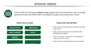
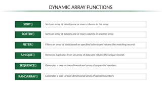
82. SORT
SORT() Sorts an array of data by one or more columns in the array
=SORT ( array, [sort_index], [sort_order], [by_col] )
An array of cells
that you want to
sort
Column # you want
to sort by
(Default is 1)
1 = Ascending
-1 = Descending
(Default is 1)
TRUE/1 = Sort by column
FALSE/0 = Sort by row
(Default is FALSE or 0)
The array in A2:D10 is being
sorted by the 4th column
(Profit) in descending order
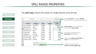
Dynamic Excel
Spill Ranges
SORT & SORTBY
FILTER
UNIQUE
SEQUENCE
RANDARRAY
Legacy Functions

83. SORT
SORT() Sorts an array of data by one or more columns in the array
Use array constants to define the
sort order for multiple columns
Dynamic Excel
Spill Ranges
SORT & SORTBY
FILTER
UNIQUE
SEQUENCE
RANDARRAY
Legacy
Functions
=SORT ( array, [sort_index], [sort_order], [by_col] )
An array of cells
that you want to
sort
Column # you want
to sort by
(Default is 1)
1 = Ascending
-1 = Descending
(Default is 1)
TRUE/1 = Sort by column
FALSE/0 = Sort by row
(Default is FALSE or 0)
The array in A2:D10 is being
sorted by the 3rd column
(Margin) in ascending order,
then the 4th column (Profit) in
descending order

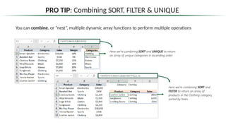
84. SORTBY
SORTBY() Sorts an array of data by one or more columns in another array
=SORTBY ( array, by_array, [sort_order], [array/order], […] )
Array of cells that
you want to sort by
1 = Ascending
-1 = Descending
(Default is 1)
Additional pairs of
arrays to sort by
This array is sorted by Profit in descending
order (even though it isn’t in the array!)
HEY THIS IS IMPORTANT!
The array you sort by must be
the same size as the array
you are sorting
Dynamic Excel
Spill Ranges
SORT & SORTBY
FILTER
UNIQUE
SEQUENCE
RANDARRAY
Legacy
Functions
An array of cells that
you want to sort

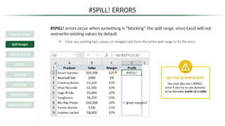
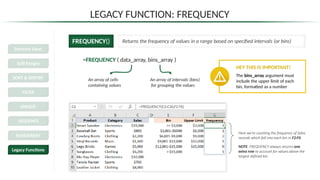
85. FILTE
R
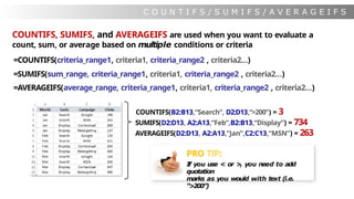
FILTER() Filters an array of data based on specified criteria and returns the matching records
=FILTER ( array, include, [if_empty] )
An array of cells that
you want to filter
A logical test to determine
the filter criteria, where
values of TRUE will be kept
An optional value to
return if nothing passes
the filter criteria
This array returns values from A2:C10,
where Category = Clothing
Dynamic Excel
Spill Ranges
SORT & SORTBY
FILTER
UNIQUE
SEQUENCE
RANDARRAY
Legacy Functions

86. FILTE
R
FILTER() Filters an array of data based on specified criteria and returns the matching records
=FILTER ( array, include, [if_empty] )
To create an AND condition between
multiple logical tests, you can
multiply them together
Dynamic Excel
Spill Ranges
SORT & SORTBY
FILTER
UNIQUE
SEQUENCE
RANDARRAY
Legacy
Functions
An array of cells that
you want to filter
A logical test to determine
the filter criteria, where
values of TRUE will be kept
An optional value to
return if nothing passes
the filter criteria
This array returns values from A2:C10 where
Category = Clothing AND Sales > 5,000
(BOTH criteria must be met)

87. FILTE
R
FILTER() Filters an array of data based on specified criteria and returns the matching records
=FILTER ( array, include, [if_empty] )
Dynamic Excel
Spill Ranges
SORT & SORTBY
FILTER
UNIQUE
SEQUENCE
RANDARRAY
Legacy
Functions
An array of cells that
you want to filter
A logical test to determine
the filter criteria, where
values of TRUE will be kept
An optional value to
return if nothing passes
the filter criteria
To create an OR condition between multiple
logical tests, you can sum them together
This array returns values from A2:C10 where
Category = Clothing OR Sales > 5,000
(EITHER criteria must be met)

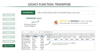
88. UNIQUE
UNIQUE() Removes duplicates from an array of data and returns only the unique records
=UNIQUE ( array, [by_col], [exactly_once] )
An array of cells that
you want to remove
duplicates from
TRUE/1 = Remove duplicates in columns
FALSE/0 = Remove duplicates in rows
(Default is FALSE or 0)
TRUE/1 = Extract values that only appear once
FALSE/0 = Extract all unique values
(Default is FALSE or 0)
This array returns the unique
Category values from B2:B10
Dynamic Excel
Spill Ranges
SORT & SORTBY
FILTER
UNIQUE
SEQUENCE
RANDARRAY
Legacy Functions

89. UNIQUE
UNIQUE() Removes duplicates from an array of data and returns only the unique records
Dynamic Excel
Spill Ranges
SORT & SORTBY
FILTER
UNIQUE
SEQUENCE
RANDARRAY
Legacy Functions
=UNIQUE ( array, [by_col], [exactly_once] )
An array of cells that
you want to remove
duplicates from
TRUE/1 = Remove duplicates in columns
FALSE/0 = Remove duplicates in rows
(Default is FALSE or 0)
TRUE/1 = Extract values that only appear once
FALSE/0 = Extract all unique values
(Default is FALSE or 0)
This array returns the Category values
from B2:B10 that appear exactly once
PRO TIP: Include multiple
columns in the array to return
each unique combination of values

90. PRO TIP: Combining SORT, FILTER & UNIQUE
You can combine, or “nest”, multiple dynamic array functions to perform multiple operations
Here we’re combining SORT and UNIQUE to return
an array of unique categories in ascending order
Here we’re combining SORT and
FILTER to return an array of
products in the Clothing category,
sorted by Sales

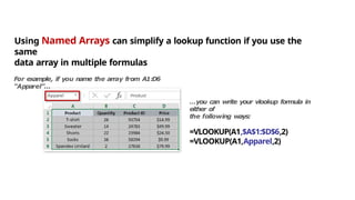
91. SEQUENCE
SEQUENCE() Generates a one- or two-dimensional array of sequential numbers
=SEQUENCE ( rows, [columns], [start], [step] )
Number of
rows to return
Number of
columns to return
Increment between each number
(Default is 1)
Starting number
(Default is 1)
This generates a 10-row, 6-column array starting at 10 and
incrementing by 5 (note the numbers go left-to-right, then down)
Dynamic Excel
Spill Ranges
SORT & SORTBY
FILTER
UNIQUE
SEQUENCE
RANDARRAY
Legacy Functions
PRO TIP: Nest SEQUENCE
within other functions to make
them more dynamic

92. RANDARRAY
RANDARRAY(
)
Generates a one- or two-dimensional array of random numbers
=RANDARRAY ( [rows], [columns], [min], [max], [integer] )
Number of
rows to return
(Default is 1)
Number of
columns to return
(Default is 1)
Minimum
value to return
(Default is 0)
Maximum
value to return
(Default is 1)
Return whole
numbers?
(Default is FALSE or 0)
This generates a 10-row by 7-column array of
random whole numbers between 0 and 100
PRO TIP: Use RANDARRAY
to randomly sort lists of data
Dynamic Excel
Spill Ranges
SORT & SORTBY
FILTER
UNIQUE
SEQUENCE
RANDARRAY
Legacy Functions

93. LEGACY FUNCTION: FREQUENCY
FREQUENCY() Returns the frequency of values in a range based on specified intervals (or bins)
=FREQUENCY ( data_array, bins_array )
An array of cells
containing values
An array of intervals (bins)
for grouping the values
Here we’re counting the frequency of Sales
records which fall into each bin in F2:F6
NOTE: FREQUENCY always returns one
extra row to account for values above the
largest defined bin
HEY THIS IS IMPORTANT!
The bins_array argument must
include the upper limit of each
bin, formatted as a number
Dynamic Excel
Spill Ranges
SORT & SORTBY
FILTER
UNIQUE
SEQUENCE
RANDARRAY
Legacy Functions

94. LEGACY FUNCTION: TRANSPOSE
TRANSPOSE() Flips a vertical range of cells to a horizontal range, or vice versa
=TRANSPOSE ( array )
An array of cells you
want to transpose
Here we’re flipping the original array in A1:C9 by
turning each column into a row
PRO TIP: Use TRANSPOSE to “pivot” your data
by turning rows into columns, or vice versa
Dynamic Excel
Spill Ranges
SORT & SORTBY
FILTER
UNIQUE
SEQUENCE
RANDARRAY
Legacy Functions

95. PRO TIP: JOINING ARRAYS WITH CHOOSE
Unique list of Categories
(using UNIQUE)
The CHOOSE function can be used to combine separate cell ranges into a single array, which can be
referenced or manipulated within other formulas
Avg Sales by Category
(using AVERAGEIF)
Raw data at the product-level
=CHOOSE({1,2},F2#,G2#)
PRO TIP: Using the array
constant {1,2} tells Excel to
combine both referenced
ranges into one dynamic array

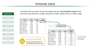
96. PRO TIP: THE LET FUNCTION
LET() Allows you to declare variables, assign values, and use them within formulas
=LET ( name1, name_value1, calculation_or_name2, [name_value2], […] )
Name of the variable
(must begin with a letter)
Value or calculation
assigned to the variable
This defines two variables, Sales and Margin,
and multiplies them to return the profit
Additional pairs of variable
names and values
A calculation using the
variable, or the name of
another variable (optional)
PRO TIP: Use LET to write clean,
efficient, user-friendly formulas

97. EXTRA BONUS FUNCTIONS

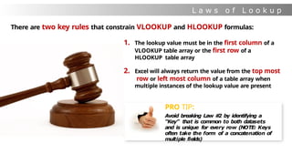
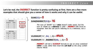
98. I N D I R E C T
The INDIRECT function returns the reference specified by a text string, and can be used
to change a cell reference within a formula without changing the formula itself
=INDIRECT(ref_text, [a1])
I
n the first ROW function, Excel
returns the row number of cell
B3, regardless of what value it
contains.
When you add INDIRECT, Excel
sees that cell B3 contains a
reference (B1) and returns the
row of the reference
ROW(B3) = 3
ROW(INDIRECT(B3)) = 1
ROW(INDIRECT(B4,0)) = 1
Which cell includes
the text that you are
evaluating?
Is your text string in A1 format (1) or R1C1 format
(0)?

99. I N D I R E C T ( c o n
t )
Let’s be real, the INDIRECT function is pretty confusing at first. Here are a few more
examples that should give you a sense of how it works and why it can be useful:
SUM(D2) = 0
SUM(INDIRECT(D2)) = 16
The sum of “B3:B5” as a value doesn’t make sense, but the
sum of B3:B5 as a reference is valid – INDIRECT tells Excel to
recognize that the cell you’re referring to is a reference, not a
value
VLOOKUP(“A”, D4, 2, 0) = #N/A
VLOOKUP(“A”, INDIRECT(D4), 2, 0) = 5
INDIRECT will tell a VLOOKUP formula to use an array contained
within a cell, rather than treat the cell itself as the array (which
returns #
N
/
A
)

100. H Y P E R L I N
K
HYPERLINK creates a shortcut that links users to a document or location within a
document (which can exist on a network server, within a workbook, or via a web
address)
=HYPERLINK(link_location,[friendly_name])
Where will people go if
they click?
How do you want the link
to read?
PRO TIP:
Use =HYPERLINK("#'"&A2&"'!A1") to jump to
cell A1 of the sheet name specified in A2
(note the extra single quotation marks!)
=HYPERLINK(”http://www.example.com/report.xlsx”, “Click Here”)
=HYPERLINK(“[C:My DocumentsReport.xlsx]”, “Open Report”)
=HYPERLINK("#Sheet2!A1”)