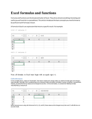
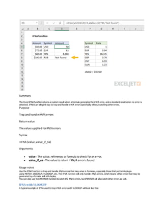
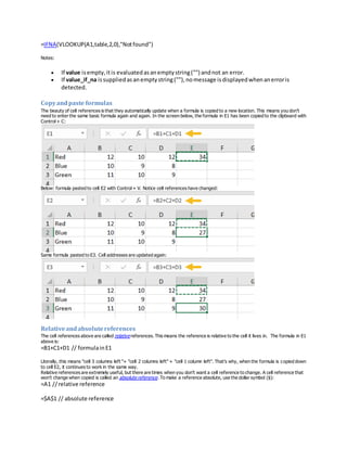
This document provides an overview of formulas and functions in Excel. It introduces the basic concepts needed to work proficiently with formulas, including how to enter formulas, use cell references, copy and paste formulas, work with relative and absolute references, and combine functions. It also covers common math operators, logical operators, and the order of operations in Excel formulas. Functions are introduced as formulas with special names and purposes, and examples are provided of commonly used functions like SUM, AVERAGE, MIN, MAX, and VLOOKUP. Tips are given for converting formulas to values and for properly structuring tables for the VLOOKUP function.
Beyond the EU: DORA and NIS 2 Directive's Global Impact
Excel formulas and functions guide
1. Excel formulas and functions
Formulasandfunctionsare the breadand butterof Excel.Theydrive almosteverythinginterestingand
useful youwill everdoina spreadsheet.Thisarticle introducesthe basicconceptsyouneedtoknowto
be proficientwith formulasinExcel.
A formulainExcel isan expressionthatreturnsaspecificresult.Forexample:
=1+2 // returns 3
=6/3 // returns 2
Note: all formulas in Excel must begin with an equals sign (=).
Cell references
In the examples above, values are "hardcoded". That means results won't change unless you edit the formula again and change a
value manually. Generally, this is considered bad form, because it hides information and makes it harder to maintain a spreadsheet.
Instead, use cell references so values can be changed at any time. In the screen below, C1 contains the following formula:
=A1+A2+A3 // returns9
Notice because we are using cell references for A1, A2, and A3, these values can be changed at any time and C1 will still show an
accurate result.
2. All formulasreturna result
All formulas in Excel return a result, even when the result is an error. Below a formula is used to calculate percent change. The
formula returns a correct result in D2 and D3, but returns a #DIV/0! error in D4, because B4 is empty:
There are different ways of handling errors. In this case, you could provide the missing value in B4, or "catch"the error with the
IFERROR function and display a more friendly message (or nothing at all).
Excel IFERROR Function
Summary
The Excel IFERROR function returns a custom result when a formula generates an error, and a standard result when no error is
detected. IFERROR is an elegant way to trap and manage errors without using more complicated nested IF statements.
Purpose
Trap and handle errors
3. Returnvalue
The value youspecifyforerrorconditions.
Syntax
=IFERROR (value,value_if_error)
Arguments
value - The value,reference,orformulatocheck foran error.
value_if_error- The value to returnif an error isfound.
Usage notes
The IFERROR function "catches"errors in a formula and returns an alternative result or formula when an error is detected.
Use the IFERROR function to trap and handle errors produced by other formulas or functions. IFERROR checks for the following
errors: #N/A, #VALUE!, #REF!, #DIV/0!, #NUM!, #NAME?, or #NULL!.
Example#1
For example, if A1 contains 10, B1 is blank, and C1 contains the formula =A1/B1, the following formula will catch the #DIV/0! error
that results from dividing A1 by B1:
=IFERROR (A1/B1,"Pleaseenteravalue inB1")
As long as B1 is empty, C1 will display the message "Please enter a value in B1" if B1 is blank or zero. When a number is ent ered in
B1, the formula will return the result of A1/B1.
Example#2
You can also use the IFERROR function to catch the #N/A error thrown by VLOOKUP when a lookup value isn't found. The syntax
looks like this:
=IFERROR(VLOOKUP(value,data,column,0),"Notfound")
In this example, when VLOOKUP returns a result, IFERROR functions that result. If VLOOKUP returns #N/A error because a lookup
value isn't found, IFERROR returns "Not Found".
Notes
If value isempty,itis evaluatedasanemptystring("") andnot an error.
If value_if_error issuppliedasanemptystring(""),nomessage isdisplayedwhenanerroris
detected.
If IFERROR isenteredasan array formula,itreturnsanarray of resultswithone itemforeach
cell in value.
In Excel 2013+, you can use the IFNA function totrap and handle #N/A errorsspecifically.
Excel IFNA Function
4. Summary
The Excel IFNA function returns a custom result when a formula generates the #N/A error, and a standard result when no error is
detected. IFNA is an elegant way to trap and handle #N/A errors specifically without catching other errors.
Purpose
Trap and handle #N/A errors
Returnvalue
The value suppliedfor#N/A errors
Syntax
=IFNA (value,value_if_na)
Arguments
value - The value,reference,orformulatocheck foran error.
value_if_na- The value toreturnif #N/A erroris found.
Usage notes
Use the IFNA function to trap and handle #N/A errors that may arise in formulas, especially those that performlookups
using MATCH, VLOOKUP, HLOOKUP, etc. The IFNA function will only handle #N/A errors, which means other errors that may be
generated by a formula will still display.
You can also use the IFERROR function to catch the #N/A errors, but IFERROR will also catch other errors as well.
IFNA with VLOOKUP
A typicalexample of IFNA used to trap #N/A errors with VLOOKUP will look like this:
5. =IFNA(VLOOKUP(A1,table,2,0),"Notfound")
Notes:
If value isempty,itis evaluatedasanemptystring("") andnot an error.
If value_if_na issuppliedasanemptystring(""),nomessage isdisplayedwhenanerroris
detected.
Copyandpaste formulas
The beauty of cell references is that they automatically update when a formula is copied to a new location. This means you don't
need to enter the same basic formula again and again. In the screen below, the formula in E1 has been copied to the clipboard with
Control+ C:
Below: formula pasted to cell E2 with Control+ V. Notice cell references have changed:
Same formula pasted to E3. Cell addresses are updated again:
Relativeandabsolutereferences
The cell references above are called relative references. This means the reference is relative to the cell it lives in. The formula in E1
above is:
=B1+C1+D1 // formulainE1
Literally, this means "cell 3 columns left "+ "cell 2 columns left"+ "cell 1 column left". That's why, when the formula is copied down
to cell E2, it continues to work in the same way.
Relative references are extremely useful, but there are times when you don't want a cell reference to change. A cell reference that
won't change when copied is called an absolute reference. To make a reference absolute, use the dollar symbol ($):
=A1 //relative reference
=$A$1 // absolute reference
6. For example, in the screen below, we want to multiply each value in column D by 10, which is entered in A1. By using an absolute
reference for A1, we "lock" that reference so it won't change when the formula is copied to E2 and E3:
Here are the final formulas in E1, E2, and E3:
=D1*$A$1 // formulainE1
=D2*$A$1 // formulainE2
=D3*$A$1 // formulainE3
Notice the reference to D1 updates when the formula is copied, but the reference to A1 never changes. Now we can easily change
the value in A1, and all three formulas recalculate. Below the value in A1 has changed from 10 to 12:
This simple example also shows why it doesn't make sense to hardcode values into a formula. By storing the value in A1 in one
place, and referring to A1 with an absolute reference, the value can be changed at any time and all associated formulas will update
instantly.
Tip: you can toggle between relative and absolute syntax with the F4 key.
Howto enter a formula
To enter a formula:
1. Selectacell
2. Enter an equalssign(=)
3. Type the formula,andpressenter.
Instead of typing cell references, you can point and click, as seen below. Note references are color-coded:
All formulas in Excel must begin with an equals sign (=). No equals sign, no formula:
7. Howto changea formula
To edit a formula, you have 3 options:
1. Selectthe cell,editinthe formulabar
2. Double-clickthe cell,editdirectly
3. Selectthe cell, pressF2,editdirectly
No matter which option you use, press Enter to confirm changes when done. If you want to cancel, and leave the formula
unchanged, click the Escape key.
Video: 20 tips for entering formulas
What is a function?
Working in Excel, you will hear the words "formula" and "function" used frequently, sometimes interchangeably. They are closely
related, but not exactly the same. Technically, a formula is any expression that begins with an equals sign (=).
A function, on the other hand, is a formula with a special name and purpose. In most cases, functions have names that reflect their
intended use. For example, you probably know the SUM function already, which returns the sum of given references:
=SUM(1,2,3) // returns6
=SUM(A1:A3) // returnsA1+A2+A3
The AVERAGE function, as you would expect, returns the average of given references:
=AVERAGE(1,2,3) // returns2
And the MIN and MAX functions return minimum and maximum values, respectively:
=MIN(1,2,3) // returns1
=MAX(1,2,3) //returns3
Excel contains hundreds of specific functions. To get started, see 101 Key Excelfunctions.
Functionarguments
Most functions require inputs to return a result. These inputs are called "arguments". A function's arguments appear after the
function name, inside parentheses, separated by commas. All functions require a matching opening and closing parentheses ().
The pattern looks like this:
=FUNCTIONNAME(argument1,argument2,argument3)
For example, the COUNTIF function counts cells that meet criteria, and takes two arguments, range and criteria:
=COUNTIF(range,criteria) //twoarguments
In the screen below, range is A1:A5 and criteria is "red". The formula in C1 is:
=COUNTIF(A1:A5,"red") //returns2
8. Video: How to use the COUNTIF function
Not all arguments are required. Arguments shown square brackets are optional. For example, the YEARFRAC function returns
fractionalnumber of years between a start date and end date and takes 3 arguments:
=YEARFRAC(start_date,end_date,[basis])
Start date and end date are required arguments, basis is an optional argument. See below for an example of how to use YEARFRAC
to calculate current age based on birthdate.
Howto enter a function
If you know the name of the function, just start typing. Here are the steps:
1. Enter equals sign (=) and start typing. Excelwill list of matching functions based as you type:
When you see the function you want in the list, use the arrow keys to select (or just keep typing).
2. Type the Tab key to accept a function. Excel will complete the function:
3. Fill in required arguments:
4. Press Enter to confirm formula:
9. Combiningfunctions(nesting)
Many Excel formulas use more than one function, and functions can be "nested" inside each other. For example, below we have a
birthdate in B1 and we want to calculate current age in B2:
The YEARFRAC function will calculate years with a start date and end date:
We can use B1 for start date, then use the TODAY function to supply the end date:
When we press Enter to confirm, we get current age based on today's date:
=YEARFRAC(B1,TODAY())
10. Notice we are using the TODAY function to feed an end date to the YEARFRAC function. In other words, the TODAY function can be
nested inside the YEARFRAC function to provide the end date argument. We can take the formula one step further and use the INT
function to chop off the decimal value:
=INT(YEARFRAC(B1,TODAY()))
Here, the original YEARFRAC formula returns 20.4 to the INT function, and the INT function returns a final result of 20.
Notes:
1. The current date in imagesabove isFebruary 22, 2019.
2. Nested IFfunctions are a classicexample of nestingfunctions.
3. The TODAY function isa rare Excel function withnorequiredarguments.
Key takeaway: The output of any formula or function can be fed directly into another formula or function.
Math Operators
The table below shows the standard math operators available in Excel:
Symbol Operation Example
+ Addition =2+3=5
- Subtraction =9-2=7
* Multiplication =6*7=42
/ Division =9/3=3
^ Exponentiation =4^2=16
() Parentheses =(2+4)/3=2
Logical operators
Logical operators provide support for comparisons such as "greater than", "less than", etc. The logical operators available in Excel
are shown in the table below:
11. Operator Meaning Example
= Equal to =A1=10
<> Notequal to =A1<>10
> Greaterthan =A1>100
< Lessthan =A1<100
>= Greaterthan or equal to =A1>=75
<= Lessthan or equal to =A1<0
Video: How to build logical formulas
Order ofoperations
When solving a formula, Excelfollows a sequence called "order of operations". First, any expressions in parentheses are evaluated.
Next Excel will solve for any exponents. After exponents, Excelwill perform multiplication and division, then addition and
subtraction. If the formula involves concatenation, this will happen after standard math operations. Finally, Excelwill evaluate
logical operators, if present.
1. Parentheses
2. Exponents
3. MultiplicationandDivision
4. AdditionandSubtraction
5. Concatenation
6. Logical operators
Tip: you can use the Evaluate feature to watch Excelsolve formulas step-by-step.
Convertformulasto values
Sometimes you want to get rid of formulas, and leave only values in their place. The easiest way to do this in Excelis to copy the
formula, then paste, using Paste Special > Values. This overwrites the formulas with the values they return. You can use a
keyboard shortcut for pasting values, or use the Paste menu on the Home tab on the ribbon.
KeyboardShortcuts
Use this shortcut to display the Paste Special dialog box. Paste Special is the gateway into many
powerful operations, including paste Values, which you probably use every day. Note that this
shortcut only works when data has been copied to the clipboard.
On Windows, once you have the Paste Special Dialog open, you can type a letter to select the
particular command you want, for example:
F = Formula
V = Values
T = Formats
C = Comments
N = Validation
12. H = All using source theme
X = All except borders
W = Column widths
R = Formulas and number formats
U = Values and number formats
D = Add
S = Subtract
M = Multiply
I = Divide
B = Skip blanks
E = Transpose
23 things you should know about VLOOKUP
When you want to pull information from a table, the Excel VLOOKUP function is a great
solution. The ability to dynamically lookup and retrieve information from a table is a game-
changer for many users, and you'll find VLOOKUP everywhere.
And yet, although VLOOKUP is a relatively easy to use, there is plenty that can go wrong. One
reason is that VLOOKUP has a major design flaw — by default, it assumes you're OK with an
approximate match. Which you probably aren't.
This can cause results that look completely normal, even though they are totally incorrect. Trust
me, this is NOT something you want to try to explain to your boss, after she's already sent your
spreadsheet to management :)
Read below learn how to manage this challenge, and discover other tips for mastering the Excel
VLOOKUP function.
1. HowVLOOKUP works
VLOOKUP is a function to lookup up and retrieve data in a table. The "V" in VLOOKUP stands
for vertical, which means the data in the table must be arranged vertically, with data in rows.
(For horizontally structured data, see HLOOKUP).
If you have a well structured table, with information arranged vertically, and a column on the left
which you can use to match a row, you can probably use VLOOKUP.
VLOOKUP requires that the table be structured so that lookup values appear in the left-most
column. The data you want to retrieve (result values) can appear in any column to the right.
When you use VLOOKUP, imagine that every column in the table is numbered, starting from the
left. To get a value from a particular column, simply supply the appropriate number as the
"column index". In the example below, we want to look up the email address, so we are using the
number 4 for column index:
13. In the above table, the employee IDs are in column 1 on the left and the email addresses are in
column 4 to the right.
To use VLOOKUP, you supply 4 pieces of information, or "arguments":
1. The value youare lookingfor(lookup_value)
2. The range of cellsthat make upthe table (table_array)
3. The numberof the columnfromwhichto retrieve aresult(column_index)
4. The match mode (range_lookup,TRUE = approximate,FALSE= exact)
Video: How to use VLOOKUP (3 min)
If you still don't get the basic idea of VLOOKUP, Jon Acampora, over at Excel Campus, has a
great explanation based on the Starbucks coffee menu.
2. VLOOKUP onlylooksright
Perhaps the biggest limitation of VLOOKUP is that it can only look to the right to retrieve data.
14. This means that VLOOKUP can only get data from columns to the right of first column in the
table. When lookup values appear in the first (leftmost) column, this limitation doesn't mean
much, since all other columns are already to the right. However, if the lookup column appears
inside the table somewhere, you'll only be able to lookup values from columns to the right of that
column. You'll also have to supply a smaller table to VLOOKUP that starts with the lookup
column.
You can overcome this limitation by using INDEX and MATCH instead of VLOOKUP.
3. VLOOKUP findsthe first match
In exact match mode, if a lookup column contains duplicate values, VLOOKUP will match the
first value only. In the example below, we are using VLOOKUP to find a first name, and
VLOOKUP is set to perform exact match. Although there are two "Janet"s in the list,
VLOOKUP matches only the first:
15. Note: behavior can change when VLOOKUP is used in approximate match mode.
How to lookup first and last match
One of the more confusing aspects of lookup functions in Excel is understanding how to get the
first or last match in a set of data with more than one match. This is because Excel's behavior
changes depending on two factors: whether you are performing an exact or approximate match,
and whether data is sorted or not.
For example, let's say we use VLOOKUP to lookup the price for "green" in the data
below. Which price will we get?
16. Read on for the answer and more interesting examples.
Notes:
The examplesbelowuse namedranges (asnotedinthe images) tokeepformulas simple.
Functionreference links: VLOOKUP,INDEX,MATCH,andLOOKUP.
Exact match = first
When doing an exact match, you'll always get the first match, period. It doesn't matter if data is
sorted or not. In the screen below, the lookup value in E5 is "red". The VLOOKUP function, in
exact match mode, returns the price for the first match:
=VLOOKUP(E5,data,2,FALSE)
Notice the last argument in VLOOKUP is FALSE to force exact match.
Approximatematch= last
If you are doing an approximate match, and data is sorted by lookup value, you'll get the last
match. Why? Because during an approximate match Excel scans through values until a value
larger than the lookup value is found, then it "steps back" to the previous value.
In the screen below, VLOOKUP is set to approximate match mode, and colors are sorted.
VLOOKUP returns the price for the last "green":
=VLOOKUP(E5,data,2,TRUE)
17. Notice the last argument in VLOOKUP is TRUE for approximate match.
Approximatematch+ unsorteddata =danger
With standard approximate match lookups, data must be sorted by lookup value. With unsorted
data, you may see normal-looking results that are totally incorrect. This problem is more likely
with VLOOKUP because VLOOKUP defaults to approximate match when no forth argument is
provided.
To illustrate this problem, see the example below. Data is unsorted and VLOOKUP, with no
forth argument provided, defaults to approximate match. Notice there is no "red" with a price of
$17.00, yet VLOOKUP happily returns this invalid result:
=VLOOKUP(E5,data,2)
18. For this reason, I recommend always setting the last argument for VLOOKUP explicitly: TRUE
= approximate match, FALSE = exact match. The argument is optional, but providing a value
makes you think about it, and provides a visual reminder in the future.
We'll look how to overcome the problem of last match and unsorted data below.
"Normal"approximatematch
At this point, you may be feeling a little confused and disoriented about the idea that
approximate match can return the last match in some cases. If so, don't worry. Using
approximate match to get the last match is not the "normal" case. Typically, you'll see
approximate match used to assign values according to some kind of scale. A classic example is
using VLOOKUP in approximate match mode to assign grades, which works beautifully:
=VLOOKUP(E5,key,2,TRUE)
19. In cases like this, the lookup table deliberately does not include duplicate values, so the whole
idea of "last matching value" is irrelevant. More details on this formula here.
The information above is to provide background and context for how matching works in Excel,
so that the approaches described below make sense.
Practical applications
How can we use the behavior described above in a practical situation? Well, one common
scenario is looking up the "latest" or "last" entry for an item. For example, below we are using
VLOOKUP in approximate match mode to find the latest price for Sandals. Notice data is sorted
by item, then by date, so the latest price for a given item appears last:
=VLOOKUP(F5,data,3,TRUE)
20. INDEXand MATCH
Other lookup functions can be used this way as well. Below, we are using an equivalent INDEX
and MATCH formula find the latest price with the same data. Notice MATCH is configured to
approximate match for items sorted in ascending order by setting the third argument to 1:
=INDEX(price,MATCH(F5,item,1))
21. LOOKUP function
The LOOKUP function can also be used in this case. LOOKUP always performs an approximate
match, so it works well in "last match" scenarios. The formula is quite simple:
=LOOKUP(F5,item,price)
Last match with unsorteddata
What if you want the last match, but data isn't sorted by lookup value? In other words, you want
to apply criteria to find a match, and you simply want the last item in the data that matches your
criteria? This is actually a case where the LOOKUP function shines, because LOOKUP can
handle array operations natively, without control + shift + enter. This means we can dynamically
build a lookup array to locate the data we want using simple logical expressions.
For example, have a look at the formula below:
=LOOKUP(2,1/(item=F5),price)
22. This formula finds the latest price for Sandals in unsorted data.
You may not have seen a formula like this before, so let's break it down in steps. Working from
the inside out, we first apply the criteria with a simple logical expression:
item=F5
This results in an array of TRUE and FALSE values, where TRUE corresponds to items that are
"sandals" and FALSE corresponds to all other values:
{FALSE;TRUE;FALSE;TRUE;FALSE;FALSE;TRUE;FALSE}
Next, we divide the number 1 by this array. During division, TRUE becomes 1 and FALSE
becomes zero, so you should visualize the operation like this:
1/{0;1;0;1;0;0;1;0}
One divided by one is one, and one divided by zero is #DIV/0, so the result is a another array,
this one containing only 1s and #DIV/0 errors:
{#DIV/0!;1;#DIV/0!;1;#DIV/0!;#DIV/0!;1;#DIV/0!}
Don't worry, there is a method to this madness :)
Now, you may have noticed that the lookup value is the number 2. This may seem
puzzling. How will LOOKUP ever find the number 2 in an array that contains only 1s and
errors? It won't. We are using 2 as a lookup value to force LOOKUP to scan to the end of the
data.
23. The LOOKUP function will automatically ignore errors, so the only thing left to match are the
1s. It will scan through the 1s looking for a 2 that will never be found. When it reaches the end of
the array, it will "step back" to the last valid value – the last 1 – which corresponds to the last
match based on criteria provided.
INDEXand MATCHarrayversion
The beauty of the LOOKUP function is it can handle the array operation described above
natively, without requiring you to enter as an array formula with control + shift + enter.
However, you can certainly use an array formula if you like. Here is the equivalent INDEX and
MATCH formula, which must be entered with control + shift + enter:
{=INDEX(price,MATCH(2,1/(item=F5),1))}
Last non-blankcell
The approach above turns out to be really useful. For example, by tweaking the logic a bit, we
can do things like find the last non-empty cell in a column:
=LOOKUP(2,1/(B:B<>""),B:B)
Excel TODAY Function
24. Summary
The Excel TODAY function returns the current date, updated continuously when a worksheet is
changed or opened. The TODAY function takes no arguments. You can format the value
returned by TODAY using any standard date format. If you need current date and time, use the
NOW function.
Purpose
Get the currentdate
Returnvalue
ValidExcel date
Syntax
=TODAY ()
Arguments
Usage notes
25. The TODAY function takes no arguments, and returns the current date, updated whenever a
worksheet is changed or opened. You can also use F9 to force the worksheet to recalculate and
update the value.
If you needa staticdate that won't change,youcan enterthe currentdate usingthe keyboard
shortcutCtrl + ;
If you needcurrentdate and time,use the NOWfunction.
Examples
=TODAY() // current date
=TODAY()-7 // one week ago
=TODAY()+7 // one week later
Formattingresults
The result of TODAY is a serial number representing a valid Excel date. You can format the
value returned by TODAY using any standard date format, or use the TEXT function to build a
text message that includes the current date.
Excel NOW Function
Summary
26. The Excel NOW function returns the current date and time, updated continuously when a
worksheet is changed or opened. The NOW function takes no arguments. You can format the
value returned by NOW as a date, or as a date with time by applying a number format.
Purpose
Get the current date and time
Return value
A serial number representing a particular date and time in Excel.
Syntax
=NOW ()
Arguments
Usage notes
NOW takes no parameters but requires empty parentheses. The value returned by NOW will
continually update each time the worksheet is refreshed (for example, each time a value is
entered or changed). Use F9 to force the worksheet to recalculate and update the value.
If you need a static time that won't change, you can enter the current time using the keyboard
shortcut Ctrl + Shift + :
Excel DAY Function
Summary
27. The Excel DAY function returns the day of the month as a number between 1 to 31 from a given
date. You can use the DAY function to extract a day number from a date into a cell. You can also
use the DAY function to extract and feed a day value into another function, like the DATE
function.
Purpose
Get the day as a number(1-31) froma date
Returnvalue
A number(1-31) representingthe daycomponentinadate.
Syntax
=DAY (date)
Arguments
date - A validExcel date.
Usage notes
The DAY function returns the day value in a given date as a number between 1 to 31 from a
given date. For example, with the date Janunary 15, 2019 in cell A1:
=DAY(A1) // returns 15
You can use the DAY function to extract a day number from a date into a cell. You can also use
the DAY function to extract and feed a day value into another function, like the DATE function.
For example, to change the year of a date in cell A1 to 2020, but leave the month and day as-is,
you can use a formula like this:
=DATE(2020,MONTH(A1),DAY(A1))
See below for more examples of formulas that use the DAY function.
Note: in Excel's date system, dates are serial numbers. January 1, 1900 is number 1 and later
dates are larger numbers. To display date values in a human-readable date format, apply a
the number format of your choice.
Notes
The date argumentmustbe a validExcel date.
Income tax bracket calculation
28. Explanation
To calculate total income tax based on multiple tax brackets, you can use VLOOKUP and a rate
table structured as shown in the example. The formula in G5 is:
=VLOOKUP(inc,rates,3,1)+(inc-VLOOKUP(inc,rates,1,1))*VLOOKUP(inc,rates,2,1)
where "inc" (G4) and "rates" (B5:D11) are named ranges, and column D is a helper column that
calculates total accumulated tax at each bracket.
Backgroundandcontext
The US Tax system is "progressive", which means people with higher taxable income pay a
higher federal tax rate. Rates are assessed in brackets defined by an upper and lower threshold.
The amount of income that falls into a given bracket is taxed at the corresponding rate for that
bracket. As taxable income increases, income is taxed over more tax brackets. Many taxpayers
therefore pay several different rates.
In the example shown, the tax brackets and rates are for single filers in the United States for the
2019 tax year. The table below shows the manual calculations for a taxable income of $50,000:
Bracket Calculation Tax
29. Bracket Calculation Tax
10% ($9,700 - $0) x 10% $970.00
12% ($39,475 - $9,700) x 12% $3,573.00
22% ($50,000-$39,475) x 22% $2,315.50
24% NA $0.00
32% NA $0.00
35% NA $0.00
37% NA $0.00
The total tax is therefore $6,858.50. (displayed as 6,859 in the example shown).
Setupnotes
1. This formula depends on VLOOKUP function in "approximate match mode". When in
approximate match mode, VLOOKUP will scan through lookup values in a table (which must be
sorted in ascending order) until a higher value is found. Then it will "step back" and return a
value from the previous row. In the event of an exact match, VLOOKUP will return results from
the matched row.
2. In order for VLOOKUP to retrieve the actual cumulative tax amounts, these have been added
to the table as a helper column in column D. The formula in D6, copied down, is:
=((B6-B5)*C5)+D5
At each row, this formula applies the rate from the row above to the income in that bracket.
3. For readability, the following named ranges, are defined: "inc" (G4) and "rates" (B5:D11).
Howthis formulaworks
In G5, the first VLOOKUP is configured to retrieve the cumulative tax at the marginal rate with
these inputs:
Lookupvalue is"inc"(G4)
Lookuptable is"rates"(B5:D11)
Columnnumberis3, Cumulative tax
Match type is1 = approximate match
30. VLOOKUP(inc,rates,3,1) // returns 4,543
With a taxable income of $50,000, VLOOKUP, in approximate match mode, matches 39,475,
and returns 4,543, the total tax up to $39,475.
The second VLOOKUP calculates the remaining income to be taxed:
(inc-VLOOKUP(inc,rates,1,1)) // returns 10,525
calculated like this:
(50,000-39,475) = 10,525
Finally, the third VLOOKUP gets the (top) marginal tax rate:
VLOOKUP(inc,rates,2,1) // returns 22%
This is multiplied by the income calculated in the previous step. The complete formula is solved
like this:
=VLOOKUP(inc,rates,3,1)+(inc-VLOOKUP(inc,rates,1,1))*VLOOKUP(inc,rates,2,1)
=4,543+(10525)*22%
=6,859
Marginal andeffectiverates
Cell G6 contains the top marginal rate, calculated with VLOOKUP:
=VLOOKUP(inc,rates,2,1) // returns 22%
The effective tax rate in G7 is total tax divided by taxable income:
=G5/inc // returns 13.7%
Note: I ran into this formula on Jeff Lenning's blog over at Excel University. It's a great example
of how VLOOKUP can be used in approximate match mode, and also how VLOOKUP can be
used multiple times in the same formula.