Downloaded 717 times
![PVTSIM FOR BEGINNERS
TABLE OF CONTENTS
1. INTRODUCTION TO PVTSIM 1
2. TYPICAL OPERATIONS IN PVTSIM 1
2.1. FLUID DATABASE CREATION – COMPOSITION BASED 1
2.2. FLUIDS FLASH OPERATION 6
2.3. FLUIDS MIXING 7
2.3.1. Case 1 Example: Gas Flow [MMSCFD], Oil Flow [STBOPD] and Water Cut [Vol%] 7
2.3.2. Case 2 Example: Min, Normal, Max Oil Flow [STBOPD], GOR [Scf/STB] & Water Cut [Vol%] 8
2.3.3. PVTSIM Simulation procedure – Mixing Operation 9
2.4. WATER SATURATION OF RESERVOIR FLUIDS (DRY BASIS) 11
2.4.1. PVTSIM Simulation procedure – Water Saturation of Reservoir Fluids (Dry Basis) 11
2.5. VISCOSITY TUNING OF OILS BASED ON LABORATORY DATA 12
2.5.1. Example Case: Gas Oil Viscosity Tuning 12
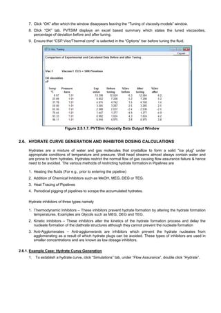
2.6. HYDRATE CURVE GENERATION AND INHIBITOR DOSING CALCULATIONS 14
2.6.1. Example Case: Hydrate Curve Generation 14
2.6.2. Example Case: Inhibitor Dosing Calculations 16
1. INTRODUCTION TO PVTSIM
PVTsim is a versatile PVT simulation program developed for reservoir engineers, flow assurance specialists, PVT
lab engineers and process engineers. Based on an extensive data collected over a period of more than 25 years,
PVTsim carries the information from experimental PVT studies into simulation software in a consistent manner
and without losing valuable information on the way. For Pipeline flow assurance studies in OLGA, PVTSIM acts as
an input to OLGA, i.e., it creates a database for the properties of selected materials with compositions,
temperature and pressure ranges, densities and viscosities. Other operations such as hydrate curves, hydrate
inhibitor dosing, wax formation, etc., can also be generated. PVTsim allows reservoir engineers, flow assurance
specialists and process engineers to combine reliable fluid characterization procedures with robust and efficient
regression algorithms to match fluid properties and experimental data. The fluid parameters may be exported to
produce high quality input data for reservoir, pipeline and process simulators.
2. TYPICAL OPERATIONS IN PVTSIM
The following typical operations are performed in PVTSim 19.2.
1. Fluid Database Creation – Composition based
2. Fluid Characterization - Based on plus fractions
3. Fluids Flashing - Fluid Property Determination
4. Fluid Mixing – for e.g. mixing of various reservoir fluids for their resultant composition
5. Water Saturation of Reservoir Fluid Compositions (dry basis) to arrive at wet composition
6. Viscosity Tuning of Oils based on Laboratory Data (e.g., ASTM D 341, Viscosity vs. Temperature)
7. Hydrate Curve Generation
8. Inhibitor Dosing and Hydrate Curve Shift study
9. Table file (*.tab) for OLGA input
2.1. FLUID DATABASE CREATION – COMPOSITION BASED
To perform various operations in PVTSim, a fluid database must be created which accepts fluid
composition. The following exercise stands essential for any case in PVTSIM.
1. Open the PVTSIM icon to get the PVTSIM user interface (Fig. 2.1.1)](https://image.slidesharecdn.com/pvtsimtraining-180529115123/85/PVTSim-Beginners-Guide-Tutorial-Multi-Phase-Calculations-1-320.jpg)
![PVTSIM FOR BEGINNERS
TABLE OF CONTENTS
1. INTRODUCTION TO PVTSIM 1
2. TYPICAL OPERATIONS IN PVTSIM 1
2.1. FLUID DATABASE CREATION – COMPOSITION BASED 1
2.2. FLUIDS FLASH OPERATION 6
2.3. FLUIDS MIXING 7
2.3.1. Case 1 Example: Gas Flow [MMSCFD], Oil Flow [STBOPD] and Water Cut [Vol%] 7
2.3.2. Case 2 Example: Min, Normal, Max Oil Flow [STBOPD], GOR [Scf/STB] & Water Cut [Vol%] 8
2.3.3. PVTSIM Simulation procedure – Mixing Operation 9
2.4. WATER SATURATION OF RESERVOIR FLUIDS (DRY BASIS) 11
2.4.1. PVTSIM Simulation procedure – Water Saturation of Reservoir Fluids (Dry Basis) 11
2.5. VISCOSITY TUNING OF OILS BASED ON LABORATORY DATA 12
2.5.1. Example Case: Gas Oil Viscosity Tuning 12
2.6. HYDRATE CURVE GENERATION AND INHIBITOR DOSING CALCULATIONS 14
2.6.1. Example Case: Hydrate Curve Generation 14
2.6.2. Example Case: Inhibitor Dosing Calculations 16
1. INTRODUCTION TO PVTSIM
PVTsim is a versatile PVT simulation program developed for reservoir engineers, flow assurance specialists, PVT
lab engineers and process engineers. Based on an extensive data collected over a period of more than 25 years,
PVTsim carries the information from experimental PVT studies into simulation software in a consistent manner
and without losing valuable information on the way. For Pipeline flow assurance studies in OLGA, PVTSIM acts as
an input to OLGA, i.e., it creates a database for the properties of selected materials with compositions,
temperature and pressure ranges, densities and viscosities. Other operations such as hydrate curves, hydrate
inhibitor dosing, wax formation, etc., can also be generated. PVTsim allows reservoir engineers, flow assurance
specialists and process engineers to combine reliable fluid characterization procedures with robust and efficient
regression algorithms to match fluid properties and experimental data. The fluid parameters may be exported to
produce high quality input data for reservoir, pipeline and process simulators.
2. TYPICAL OPERATIONS IN PVTSIM
The following typical operations are performed in PVTSim 19.2.
1. Fluid Database Creation – Composition based
2. Fluid Characterization - Based on plus fractions
3. Fluids Flashing - Fluid Property Determination
4. Fluid Mixing – for e.g. mixing of various reservoir fluids for their resultant composition
5. Water Saturation of Reservoir Fluid Compositions (dry basis) to arrive at wet composition
6. Viscosity Tuning of Oils based on Laboratory Data (e.g., ASTM D 341, Viscosity vs. Temperature)
7. Hydrate Curve Generation
8. Inhibitor Dosing and Hydrate Curve Shift study
9. Table file (*.tab) for OLGA input
2.1. FLUID DATABASE CREATION – COMPOSITION BASED
To perform various operations in PVTSim, a fluid database must be created which accepts fluid
composition. The following exercise stands essential for any case in PVTSIM.
1. Open the PVTSIM icon to get the PVTSIM user interface (Fig. 2.1.1)](https://image.slidesharecdn.com/pvtsimtraining-180529115123/75/PVTSim-Beginners-Guide-Tutorial-Multi-Phase-Calculations-1-2048.jpg)

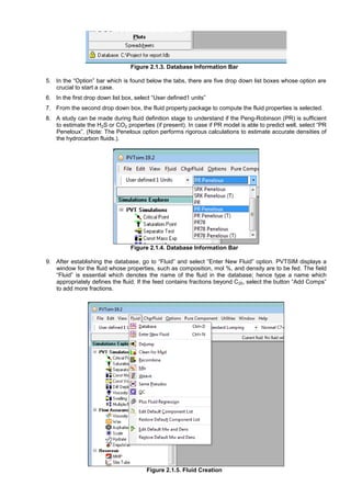
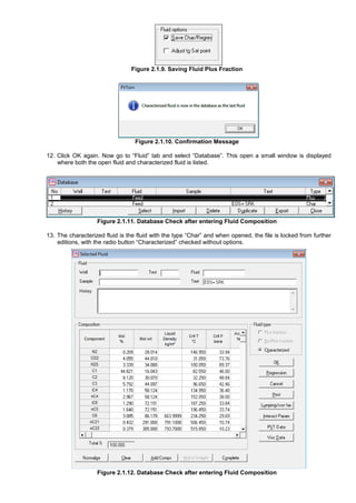
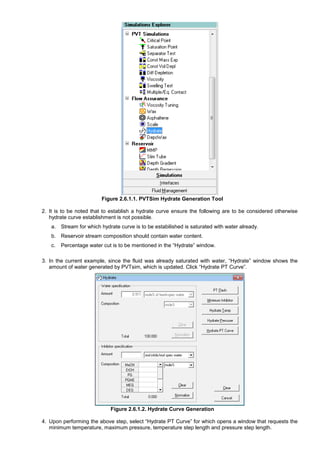
![Figure 2.2.2. Flash Operation Output Window
2.3. FLUIDS MIXING
If the reservoir data supplied contains more then one reservoir fluid fluids, then it becomes essential to mix
them, if the combined properties are required. i.e., Individual reservoir compositions have to be mixed in the
various fractions to arrive at a single stream. Often reservoir data is provided in terms of expected fluids
production versus time (years). The reservoir production data is provided in two formats as shown below.
1. Case 1: Gas Flow [MMSCFD], Oil Flow [STBOPD] and Water Cut [Wt% or Vol%]
2. Case 2: Min, Normal, Max Oil Flow [STBOPD] with GOR [Scf/STB] and Water Cut [Wt% or Vol%]
2.3.1. Case 1 Example: Gas Flow [MMSCFD], Oil Flow [STBOPD] and Water Cut [Vol%]
For a given year,, the following production flow rates are expected. Calculate the individual mass fractions of
each component and the total mass flow expected for the year in question
Table 2.3.1.1. Case 1: Example Production Profile
Example Case 1: Production Profile
Note 1
Year
Oil Rate Gas Rate Water Cut
[STBOPD] [MMSCFD] [Vol%]
2020 25,000 40 12
Standard Density
Note 2
Year
Oil Density Gas Density Water Density
[Std. kg/m
3
] [Std. kg/m
3
] [Std. kg/m
3
]
2020 850 1.2 1,000
Note 1: 1 Barrel (oil)/ hour = 4.4163137×10
-5
m
3
/s
Note 2: In the example production profile (Table 2.3.1.1); the densities are given at standard conditions as the
individual flow rates are also given at standard conditions. In practice, the standard density or actual density must be
appropriately chosen depending on the conditions of the input flow rates to calculate the volumetric flow rates.](https://image.slidesharecdn.com/pvtsimtraining-180529115123/85/PVTSim-Beginners-Guide-Tutorial-Multi-Phase-Calculations-7-320.jpg)
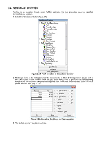
![Therefore from table 2.3.1.1, the individual mass flows are computed as,
1. Oil Mass Flow = sQ OilOil kg1027.39850104163137.4
24
25000 5
2. Gas Mass Flow = sQ GasGas kg7316.151.2107.8657907
24
1040 6-
6
3. Water Volume Flow STBOPDW
W
W
5682
25000
12.0
4. Water Mass Flow = sQ WaterWater kg4556.100001104163137.4
24
5682 5
Therefore the mass fraction of individual fluids is as follows,
Table 2.3.1.2. Case 1 Example: Calculated Mass Fractions
Mass Fractions
Year 2020 Units Oil Gas Water Total
Mass Flow kg/s 39.1027 15.7316 10.4556 65.2899
Mass Fraction [-] 0.5989 0.2409 0.1601 1.0000
2.3.2. Case 2 Example: Min, Normal, Max Oil Flow [STBOPD], GOR [Scf/STB] & Water Cut [Vol%]
For a given year, the following production flow rates are expected. Calculate the individual mass fractions of
each component and the total mass flow expected for the Year 2020.
Table 2.3.2.1. Case 2: Example Production Profile
Example Case 2: Production Profile
Note 1
Year
Minimum Normal Maximum Water Cut GOR
[STBOPD] [STBOPD] [STBOPD] [Vol%] [Scf/STB]
2020 8,000 10,000 12,000 12 2,200
Standard Density
Note 2
Year
Oil Density Water Density Gas Density
[Std. kg/m
3
] [Std. kg/m
3
] [Std. kg/m
3
]
2020 850 1,000 1.2
Note 1: 1 Barrel (oil)/ hour = 4.4163137×10
-5
m
3
/s
Note 2: In the example production profile (Table 2.3.1.1); the densities are given at standard conditions as the
individual flow rates are also given at standard conditions. In practice, the standard density or actual density must be
appropriately chosen depending on the conditions of the input flow rates to calculate the volumetric flow rates.
Therefore from table 2.3.2.1, the individual mass flows are computed as,
1. Minimum Oil Mass Flow = sQ OilOil kg5129.12850104163137.4
24
8000 5
2. Normal Oil Mass Flow = sQ OilOil kg6411.15850104163137.4
24
10000 5
3. Maximum Oil Mass Flow = sQ OilOil kg7693.18850104163137.4
24
12000 5
4. Water Volume Flow STBOPDW
W
W
5682
25000
12.0
5. Water Mass Flow = sQ WaterWater kg4556.100001104163137.4
24
5682 5
](https://image.slidesharecdn.com/pvtsimtraining-180529115123/85/PVTSim-Beginners-Guide-Tutorial-Multi-Phase-Calculations-8-320.jpg)
![The mass flow of gas is computed as,
6.
Std
OilOilOilOilGas
m
kg
Day
STB
Q
STB
Sm
STB
Scf
GORQGORM
3
3
70.02831684
Therefore the mass flow of gas is computed for minimum, normal and maximum conditions as,
7. skg
m
kg
Day
STB
STB
Sm
M
Std
MinGas 9219.6
360024
1
2.1800070.028316842200 3
3
,
8. skg
m
kg
Day
STB
STB
Sm
M
Std
NorGas 6524.8
360024
1
2.11000070.028316842200 3
3
,
9. skg
m
kg
Day
STB
STB
Sm
M
Std
MaxGas 3828.10
360024
1
2.11200070.028316842200 3
3
,
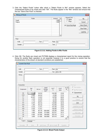
Using the various oil, gas and water mass flow rates computed, the mass fractions for the minimum, normal
and maximum water conditions are estimated as follows,
Table 2.3.1.2. Case 2 Example: Calculated Mass Fractions
Mass Fractions - Minimum Case
Year 2020 Units Oil Gas Water Total
Mass Flow kg/s 12.5129 6.9219 10.4556 29.8904
Mass Fraction [-] 0.4186 0.2316 0.3498 1.0000
Mass Fractions - Normal Case
Year 2020 Units Oil Gas Water Total
Mass Flow kg/s 15.6411 8.6524 10.4556 34.7491
Mass Fraction [-] 0.4501 0.2490 0.3009 1.0000
Mass Fractions - Maximum Case
Year 2020 Units Oil Gas Water Total
Mass Flow kg/s 18.7693 10.3828 10.4556 39.6077
Mass Fraction [-] 0.4739 0.2621 0.2640 1.0000
2.3.3. PVTSIM Simulation procedure – Mixing Operation
Based on the calculations made in the previous sections and taking case 1 as an example study, the mixing
operation is performed as follows,
1. Click the “Fluid Management” tab, under “Fluid” and double click “Mix”. PVTSIM now displays “Mixing of
fluids” window.
2. The different fluids can be mixed in terms of molar fraction or mass fraction.
Figure 2.3.3.1. Mixing of Fluids Input Window](https://image.slidesharecdn.com/pvtsimtraining-180529115123/85/PVTSim-Beginners-Guide-Tutorial-Multi-Phase-Calculations-9-320.jpg)
![2.5. VISCOSITY TUNING OF OILS BASED ON LABORATORY DATA
Though PVTSIM generates viscosities for oils at desired process conditions, the predicted viscosities
sometimes are erroneous. PVTSIM provides an option to match the viscosities with laboratory data.
2.5.1. Example Case: Gas Oil Viscosity Tuning
The viscosity curve for a certain finished product namely Gas Oil with the following composition (Table
2.5.1.1) is shown in Fig. 2.5.1.1. Using this data, the gas oil viscosity in PVTSim needs to be tuned with that
of the Laboratory ASTM D 341 Curve.
Table 2.5.1.1. Example Case: Gas Oil Composition
Gas Oil Property Estimation (Density @ 15.6 C - 860.5 kg/m
3
)
Component Mol % Mol Fraction Mol wt Liquid Density [kg/m³]
C8 1 0.01 107 765
C9 1 0.01 121 781
C10 1 0.01 134 792
C11 1 0.01 147 796
C12 3 0.03 161 810
C13 5 0.05 175 825
C14 5 0.05 190 836
C15 19.5 0.195 206 842
C16 18.5 0.185 222 850
C17 45 0.45 237 884
Note1
Note 1: C17 fraction is not a plus fraction
The ASTM D 341 Kinematic Viscosity versus Temperature Curve is as follows,
Table 2.5.1.2. Viscosity vs.
Temperature
ASTM D 341 K.V vs. T
Temperature K. Viscosity
[F] [C] [cSt]
45 7.22 14
50 10.00 12.5
75 23.89 8
100 37.78 5.50
125 51.67 4.00
150 65.56 3.00
175 79.44 2.50
200 93.33 2.00 Figure 2.5.1.1. ASTM D 341 Kinematic Viscosity vs. Temperature
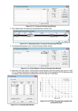
Therefore to tune the viscosities with respect to Laboratory data, the following procedure is employed.
1. Obtain Laboratory data, e.g., ASTM D 341 Kinematic Viscosity versus Temperature Curve (Fig. 2.5.1.1)
2. PVTSIM requires temperature in Celsius, pressure in Bara and dynamic viscosity in cP (Table 2.5.1.2)
3. In the “Simulation” tab, under “Flow Assurance”, double click “Viscosity Tuning”. A window named
“Tuning of viscosity models” is displayed.](https://image.slidesharecdn.com/pvtsimtraining-180529115123/85/PVTSim-Beginners-Guide-Tutorial-Multi-Phase-Calculations-12-320.jpg)
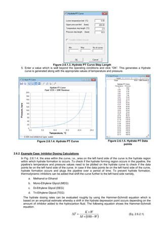
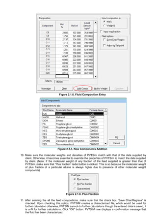
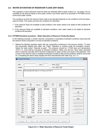
![Where,
T = Temperature shift, hydrate depression [°F]
K = Constant [-] which is defined in the Table 2.6.2.1
W = Mass of inhibitor in kg/ kg water or weight% inhibitor in aqueous phase
M = Molecular weight of the inhibitor
The constant K defined for various thermodynamic inhibitors is as follows,
Table 2.6.2.1. Inhibitor Constants in Hammer-Schmidt Equation
INHIBITOR K
Methanol 2335
Ethanol 2335
Mono-Ethylene Glycol 2700
Di-Ethylene Glycol 4000
Tri-Ethylene Glycol 5400
The Hammer-Schmidt equation was generated based upon more than 100 natural gas hydrate
measurements with inhibitor concentrations of 5 to 25 wt% in water. The accuracy of the equation is 5%
average error compared with 75 data points. Considering a 10
0
C temperature shift, the inhibitor dosing can
be calculated for various thermodynamic inhibitors by re-arranging eq. 2.6.2.2 as,
M
T
K
M
W
100
(Eq. 2.6.2.2)
Table 2.6.2.2. Inhibitor Dosing calculations
Inhibitor Methanol Ethanol MEG DEG TEG
Molecular Formula CH3OH C2H5OH C2H6O2 C4H10O3 C6H14O4
Molecular Weight 32.04 46.07 62.07 106.12 150.17
Constant [K] 2335 2335 2700 4000 5400
T [
0
F] 10 10 10 10 10
W (Weight% Inhibitor) 40.69 49.66 53.48 57.02 58.17
From the above table, it can be concluded that Methanol is the inhibitor required in lower quantities and
TEG is required approximately twice the amount of Methanol, i.e., Methanol has a higher temperature shift
than the glycols, but MEG has a lower volatility than methanol and MEG may be recovered and recycled
more easily than methanol on platforms. The above calculations can be entered into PVTSim in the Inhibitor
specification window as follows,
Figure 2.6.2.1. Inhibitor Dosing Window](https://image.slidesharecdn.com/pvtsimtraining-180529115123/85/PVTSim-Beginners-Guide-Tutorial-Multi-Phase-Calculations-17-320.jpg)

The document serves as a beginner's guide to the pvtsim software, detailing its operations for reservoir engineers and fluid characterization specialists. It outlines typical operations such as fluid database creation, flash operations, mixing fluids, and water saturation of reservoir fluids. Additionally, it explains the process for viscosity tuning and generating hydrate curves, emphasizing the importance of accurately defining fluid properties for effective simulation.