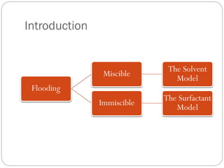
This document provides an overview of the solvent and surfactant models in reservoir simulation. It discusses the objectives and applications of the solvent model, which models miscible displacement processes. It describes the Todd & Longstaff model for representing miscibility and outlines how to treat relative permeability and PVT data. It then discusses the surfactant model, how it models surfactant distribution and its effects on water viscosity, capillary pressure, relative permeability and adsorption.

1. Prepared by:
Group 5
The Solvent & Surfactant Models
KhaledAl Shater
Mohamed Sherif Mahrous
Ramez Maher Aziz
Ahmed Kamal Khalil
George Ashraf
HazemAL Nazer
Hameda Abd-Elmawla Mahdi

2. Agenda
 Introduction
 The Solvent Model
 Objectives of the Solvent Model
 Applications of the Solvent Model
 Todd & Longstaff Model
 DataTreatment for Using the Solvent Model
 The Surfactant Model
 Introduction & Application
 Surfactant Distribution
 DataTreatment for Using the Surfactant Model

3. Introduction
Flooding
Miscible
The Solvent
Model
Immiscible
The Surfactant
Model

4. The Solvent Model
The Solvent Model

5. Objectives of the Solvent Model
 The aim of this chapter is to enable modeling of reservoir
recovery mechanisms in which injected fluids are miscible
with the hydrocarbons in the reservoir.
 A miscible displacement has the advantage over immiscible
displacements such as water flooding, of enabling very high
recoveries.An area swept by a miscible fluid typically leaves a
very small residual oil saturation.
 The ECLIPSE solvent extension allows you to model gas
injection projects without going to the complexity and
expense of using a compositional model
 In Eclipse, the solvent extension implements theTodd and
Longstaff empirical model for miscible floods.

6. Applications of the Solvent Model
 The solvent model is used in any scheme in which the aim is to
enhance the reservoir sweep by using a miscible injection fluid.
Examples of solvent schemes are listed below:
1. High pressure dry gas processes, in which miscible flow conditions
between the gas and the oil are found at the gas-oil contact .
2. A solvent such as LPG or propane may be injected as a‘slug’ to be
followed by an extended period of lean gas injection.The slug fluid
is miscible with both the gas and oil.
3. Certain non-hydrocarbon gases such as carbon dioxide produce
miscible displacement of oil at pressures above a threshold value.
4. All-liquid miscible displacements by fluids such as alcohol,
normally injected as a slug between the in-place oil and the injected
chase water.

7. Todd & Longstaff Model
 In Eclipse, the solvent extension implements theTodd and Longstaff
empirical model for miscible floods.
 The model classifies the reservoir into 3 possible miscibility combinations:
1. In regions of the reservoir containing only solvent and reservoir oil (possibly
containing dissolved gas) the solvent and reservoir oil components are
assumed to be miscible in all proportions and consequently only one
hydrocarbon phase exists in the reservoir.The relative permeability
requirements of the model are those for a two phase system
(water/hydrocarbon).
2. In regions of the reservoir containing only oil and reservoir gas, the gas and
oil components will be immiscible and will behave in a traditional black oil
manner.
3. In regions containing both dry gas and solvent, an intermediate behavior is
assumed to occur, resulting in an immiscible/miscible transition region.

8. Todd & Longstaff Mixing Parameter ω
 The model introduces an empirical parameter, ω, whose value lies between 0
and 1, to represent the size of the dispersed zone in each grid cell.The value of
ω thus controls the degree of fluid mixing within each grid cell.
 A value of ω = 1 models the case when the size of the dispersed zone is much
greater than a typical grid cell size and the hydrocarbon components can be
considered to be fully mixed in each cell.
 A value of ω = 0 models the effect of a negligibly thin dispersed zone between
the gas and oil components, and the miscible components should then have the
viscosity and density values of the pure components. In practical applications an
intermediate value of ω would be needed to model incomplete mixing of the
miscible components.
 An intermediate value of ω results in a continuous solvent saturation increase
behind the solvent front.Todd and Longstaff accounted for the effects of viscous
fingering in 2D studies by setting ω = 2 /3 independently of mobility ratio. For
field scale simulations they suggested setting ω = 1 /3 . However, in general
history matching applications, the mixing parameter may be regarded as a useful
history matching variable to account for any reservoir process inadequately
modeled.

9. Data Treatment for Using the Solvent Model
 The main differences between using the black oil simulator
without the solvent model and using it with the solvent
model are:
i. Phases present.
ii. Relative permeability data treatment.
iii. PVT data treatment.

10. I. Phases Present
 To initiate the Solvent model, the following keywords must
be added to RUNSPEC section:

11. II. Relative Permeability Data Treatment
Relative permeability data treatment depends on whether the
displacement in the grids concerned is:
1. Fully miscible
2. Fully immiscible
3. Transition between miscible and immiscible regimes

12. 1. In case of fully miscible:
In regions where solvent is displacing oil and the reservoir gas
saturation is small, the hydrocarbon displacement is miscible.
However, the 2-phase character of the water/hydrocarbon
displacement needs to be taken into account.The relative
permeabilities are given by:

13. 2. In case of fully immiscible:
In the usual black-oil model the relative permeabilities for the
3 phases water, oil and gas are specified as follows:

14. 2. In case of fully Immiscible:
When two gas components are present, the assumption is made
that the total relative permeability of the gas phase is a function
of the total gas saturation,
Then the relative permeability of either gas component is taken
as a function of the local solvent fraction within the gas phase,

15. 3. In case of Transition between
miscible and immiscible:
The transition algorithm has two steps:
1. Scale the relative permeability end points by the miscibility
function. For example, the residual oil saturation is
2. Calculate the miscible and immiscible relative
permeabilities, scaling for the new end points.Then the
relative permeability is again an interpolation between the
two using the miscibility function:

16. III. PVT Data Treatment
The PVT data treatment is made for:
1. Viscosity
2. Density

17. 1. Viscosity data treatment:
The following form is suggested byTodd and Longstaff for the
effective oil and solvent viscosities to be used in an immiscible
simulator.

18. 1. Viscosity data treatment:
The mixture viscosities μmos , μmsg and μum are defined
using the 1/4th-power fluid mixing rule, as follows:

19. 2. Density data treatment:
The effective oil and solvent densities (ρo eff , ρs eff , ρg eff )
are now computed from the effective saturation fractions and
the pure component densities (ρo , ρs , ρg ) using the
following formulae:

20. 2. Density data treatment:
The effective saturation fractions are calculated from:

21. The Surfactant Model
The Surfactant Model

22. Introduction & Application
 Most large oil fields are now produced with water-flooding
to increase recovery oil, but there’s a large volume of
unrecovered oil.
 The remaining oil can be divided into two classes:
o Residual oil to the water flood
o Oil bypassed by the water flood
 A surfactant flood is a tertiary recovery mechanism aimed at
reducing the residual oil saturation in water swept zones

23.  The oil becomes immobile because of the surface tension
between oil and water; the water pressure alone is unable to
overcome the high capillary pressure required to move oil
out of very small pore volumes.
 A surfactant reduces the surface tension, hence reduces
capillary pressure and allows water to displace extra oil.
Introduction & Application

24. The surfactant Model
 To modelThe surfactant, we need to calculate:
 Its distribution at each grid block
 Its effect on:
 Water PVT data (Viscosity of water-surfactant mixture).
 SCAL data (Capillary pressure, Relative permeability,Wettability).

25. Surfactant Distribution
 The surfactant is assumed to exist only in the water phase not
as a separate phase.
 The user inputs the concentration of surfactant in the
injection stream of each well.
 The distribution of injected surfactant is modeled by solving
a conservation equation for surfactant within the water
phase.

26. Water PVT properties
 The surfactant modifies the viscosity of the pure or salted
water.
 The surfactant viscosity is inputted as a function of surfactant
concentration.
 The water-surfactant solution viscosity calculated by:

27. Water PVT properties
 If the Brine option is active, it’s calculated as:
 Where:

28. SCAL data
 The Surfactant effects various SCAL data like:
Capillary pressure, Relative permeability,Wettability
 To Study its effect we need to input tables of water-oil
surface tension as a function of surfactant concentration in
the water using (keyword SURFACT)

29. Calculation of the capillary number
 The capillary number the ratio of viscous forces to capillary
forces.The capillary number is calculated by:

30. The Relative Permeability model
 The Relative Permeability model is essentially a transition
from immiscible relative permeability curves at low capillary
number to miscible relative permeability curves at high
capillary number.You supply a table that describes the
transition as a function of log10(capillary number).
 The relative permeability used at a value of the miscibility
function between the two extremes

31. The Relative Permeability model

32. Capillary pressure
 The water oil capillary pressure will reduce as the
concentration of surfactant increases and hence decreases the
residual oil saturation.
 The oil water capillary pressure is calculated by:

33. Treatment of adsorption
 The tendency of the surfactant to be adsorbed by the rock
will influence the success or failure of a surfactant flood
 If the adsorption is too high, then large quantities of
surfactant will be required to produce a small quantity of
additional oil.
 The quantity adsorbed is a function of the surrounding
surfactant concentration.
 To model it,The user is required to supply an adsorption
isotherm as a function of surfactant concentration

34. Treatment of adsorption
 The quantity of surfactant adsorbed on to the rock is given
by: Matrix density

35. List of References:
1. EclipseTechnical Description Manuel, Chapters 62 & 64.
2. Todd, M.R. Longstaff,W.J, 1972. The Development,Testing,
and Application Of a Numerical Simulator for Predicting Miscible
Flood Performance. J. Pet.Technol, 24(6): 874-882

36. Thank You