This document provides guidelines for sizing an anti-surge valve for a centrifugal compressor. It begins with definitions of surge and how it can damage compressors. It then outlines the methodology for sizing an anti-surge valve, which involves calculating the valve coefficient based on parameters like mass flow rate, pressure ratio, piping geometry, and gas properties. The document provides a case study applying this methodology to size a 4" anti-surge valve for a gas compressor system operating between 11.61 and 30.13 bara.

1. Page 1 of 8
Design Considerations for Antisurge Valve Sizing
Jayanthi Vijay Sarathy, M.E, CEng, MIChemE, Chartered Chemical Engineer, IChemE, UK
Centrifugal Compressors experience a
phenomenon called “Surge” which can be
defined as a situation where a flow reversal
from the discharge side back into the
compressor casing causing mechanical
damage.
The reasons are multitude ranging from
driver failure, power failure, upset process
conditions, start up, shutdown, failure of anti-
surge mechanisms, check valve failure to
operator error to name a few. The
consequences of surge are more mechanical
in nature whereby ball bearings, seals, thrust
bearing, collar shafts, impellers wear out and
sometimes depending on the how powerful
are the surge forces, cause fractures to the
machinery parts due to excessive vibrations.
The following tutorial explains how to size an
anti-surge valve for a single stage VSD system
for Concept/Basic Engineering purposes.
General Notes & Assumptions
1. Centrifugal compressors are characterized
by “Performance curves” which are a plot
of Actual Inlet Volumetric Flow rate [Q] vs.
Polytropic head [Hp] for various operating
speeds. The operating limits for
performance curves are the surge line and
the choke flow line, beyond which any
compressor operation can cause severe
mechanical damage.
2. Below is an image of performance curves
characteristics which indicates the surge
flow line and choked flow line, both of
which extend from the minimum speed Q
vs. Hp curve to the maximum speed Q vs. Hp
curve. The surge curve is defined as the
Surge Limit Line [SLL] and an operating
margin is provided [e.g., 10% on flow rate]
which is called the surge control line [SCL].
Figure 1. Performance Curves Operating Limits [1]
3. To ensure process safety & avoid
mechanical damage, the anti-surge valve
(ASV) must be large enough to recycle flow
sufficiently. An undersized valve would fail
to provide enough recycle flow to keep the
compressor operating point away from SCL
and SLL. Whereas over sizing the ASV leads
to excess gas recycling that can drive the
compressor into the choke flow region.
Oversized valves also create difficulties in
tuning the controllers due to large
controller gain values and limited stroke.
Figure 2. Sizing Criteria for Anti-surge Valve
4. To size the anti-surge valve (ASV), the
philosophy employed should consider,
operating the compressor on the right
hand side of the SCL while also ensuring

2. Page 2 of 8
the operating point does not cross the
choke flow line. Towards this, the recycle
flow rates across the ASV can be taken to
be 1.8 to 2.2 times the surge flow rate.
5. Traditionally ASVs have linear opening
characteristics, though sometimes equal
percentage characteristics can be
incorporated into the linear trend. Quick
opening characteristics are not preferred
due to poor throttling characteristics while
Equal percentage valves suffer from slow
opening during the early travel period.
6. The stroking time of the valve should be
ideally less than 2 sec with less than 0.4 sec
time delay and no overshoot. The actuator
response time must be less than 100 msec
and the noise limit is ~85 dBA. The
maximum noise level allowed is 110 dBA.
7. Anti-surge valves are Fail-open [FO] type
and should provide stable throttling. Fluid
velocities should be less than 0.3 Mach to
avoid piping damage and valve rattling.
8. The anti-surge valve can be operated
pneumatically or by solenoid action. For
valve sizes greater than 16”, a motor
operated valve can be used to effectuate
the fast opening requirements.
9. Although the current tutorial provides a
methodology to size an ASV which is
suitable during Concept/Basic Engineering
stage, a compressor dynamic simulation
shall be performed with the actual plant
layout based on detailed design to verify if
the ASV can cater to preventing a surge
during start-up & shutdown scenarios.
10. The final ASV size must be verified and
arrived in concurrence with the
turbomachinery vendor, valve
manufacturer, if the ASV can cater to the
surge control philosophy employed, slope
of the performance curves and polytropic
efficiency maps at the choke points.
Anti-Surge Valve Sizing Methodology
To size the anti-surge valve, the ANSI/ISA
S75.01 compressible fluid sizing expression is
chosen for this exercise and the flow rates are
taken for at least 1.8 to 2.2 times the surge
flow rate.
Step 1: Calculate Piping Geometry (Fp)
𝐹𝑃 = [1 +
∑ 𝐾
890
(
𝐶 𝑉
𝑑2
)
2
]
−1
2⁄
(1)
Where,
Fp = Piping geometric Factor [-]
Cv = Valve Coefficient [-]
d = Control Valve Size [inch]
K = Sum of Pipe Resistance Coefficients [-]
The value of Fp is dependent on the fittings
such as reducers, elbows or tees that are
directly attached to the inlet & outlet
connections of the control valve. If there are
no fittings, Fp is taken to be 1.0. The term K
is the algebraic sum of the velocity head loss
coefficients of all the fittings that are attached
to the control valve & is estimated as,
∑ 𝐾 = 𝐾1 + 𝐾2 + 𝐾 𝐵1−𝐾 𝐵2 (2)
Where,
K1 = Upstream fitting resistance coefficient [-]
K2 = Downstream resistance coefficient [-]
KB1 = Inlet Bernoulli Coefficient [-]
KB2 = Outlet Bernoulli Coefficient [-]
Where,
𝐾 𝐵1 = 1 − (
𝑑
𝐷1
)
4
(3)
𝐾 𝐵2 = 1 − (
𝑑
𝐷2
)
4
(4)
Where,
D1 = Inlet Pipe Inner Diameter [in]
D2 = Outlet Pipe Inner Diameter [in]
The most commonly used fitting in control
valve installations is the short-length
concentric reducer. The expressions are as
follows,

3. Page 3 of 8
𝐾1 = 0.5 × [1 − (
𝑑2
𝐷1
2)]
2
, for inlet reducer (5)
𝐾2 = 1.0 × [1 − (
𝑑2
𝐷2
2)]
2
, for outlet reducer (6)
Step 2: Calculate Valve Coefficient (Cv)
To calculate the valve Cv, the following
ANSI/ISA expression is used.
𝐶𝑣 =
𝑀
𝑁8 𝐹𝑝 𝑃1 𝑌√
𝑋×𝑀𝑊
𝑇1×𝑍
(7)
𝑋 =
∆𝑃
𝑃1
(8)
𝑌 = 1 −
𝑋
3×𝐹 𝑘×𝑋 𝑇
(9)
𝐹𝑘 =
𝑘1
1.4
(10)
If X > Fk  XT, then flow is Critical.
If X < Fk  XT, then flow is Subcritical.
For Critical flow, the value of ‘X’ is replaced
with Fk  XT and the gas expansion Factor [Y]
and valve coefficient [Cv] is to be computed as,
𝑌 = 1 −
𝐹 𝑘×𝑋 𝑇
3×𝐹 𝑘×𝑋 𝑇
= 0.667 (11)
𝐶𝑣 =
𝑀
0.667×𝑁8 𝐹𝑝 𝑃1√
𝐹 𝑘×𝑋 𝑇×𝑀𝑊
𝑇1×𝑍
(12)
If the control valve inlet and outlet piping is
provided with reducers and expanders, then
the value of XT is replaced with XTP as follows,
𝑋 𝑇𝑃 =
𝑋 𝑇
𝐹𝑝
2 × [1 +
𝑋 𝑇(𝐾1+𝐾 𝐵1)
1000
(
𝐶 𝑣
𝐷1
2)
2
]
−1
(13)
Where,
Cv = Cv value at Valve 100% Open [-]
M = Mass Flow Rate [kg/h]
N8 = Constant [Value = 94.8]
Fp = Piping Geometry Factor [-]
P = Pressure drop across ASV [bar]
P1 = Inlet Pressure [bara]
Y = Gas Expansion Factor [-]
X = Pressure Drop Ratio [-]
Z = Gas compressibility Factor [-]
T1 = Inlet Temperature [K]
Fk = Gas specific heat to air specific heat ratio
k1 = Gas specific heat ratio at valve inlet [-]
XTP and XT = Pressure drop ratio factor [-]
MW = Molecular Weight of gas [kg/kmol]
To estimate the compressor mass flow rate
from the suction density [s] and compressor
actual inlet flow rate, it can be estimated as,
𝜌𝑠 =
𝑃×𝑀𝑊
𝑍×𝑅×𝑇
(14)
𝑀 = 𝑄𝑠 × 𝜌𝑠 (15)
Where,
R = Gas Constant [0.0831447 m3.bar/kmol.K]
Qs = Compressor Suction Vol flow rate [m3/h]
To arrive at a converged value of Fp, the valve
Cv at each iteration, can be computed
iteratively by replacing the Fp value in each
iteration of the Cv equation. Applying the
Sizing method, to the four points shown in
Figure 2, the various sizing scenarios are,
a. Minimum Speed - Surge Flow [Q1]
b. Minimum Speed - Surge Flow [Q1  1.8]
c. Minimum Speed - Surge Flow [Q1  2.2]
d. Maximum Speed - Surge Flow [Q2]
e. Maximum Speed - Surge Flow [Q2  1.8]
f. Maximum Speed - Surge Flow [Q2  2.2]
g. Minimum Speed - Choke Flow [Q3]
h. Maximum Speed - Choke Flow [Q4]
The ASV Cv computed for the surge points
would be closer to each other in most cases.
Similarly, the ASV Cv at the choke points
would also be closer to each other. Therefore,
to arrive at conservative results, the higher of
the Cv values at the surge points & the lower
of the Cv values at the choke points are to be
considered to determine a suitable ASV size.

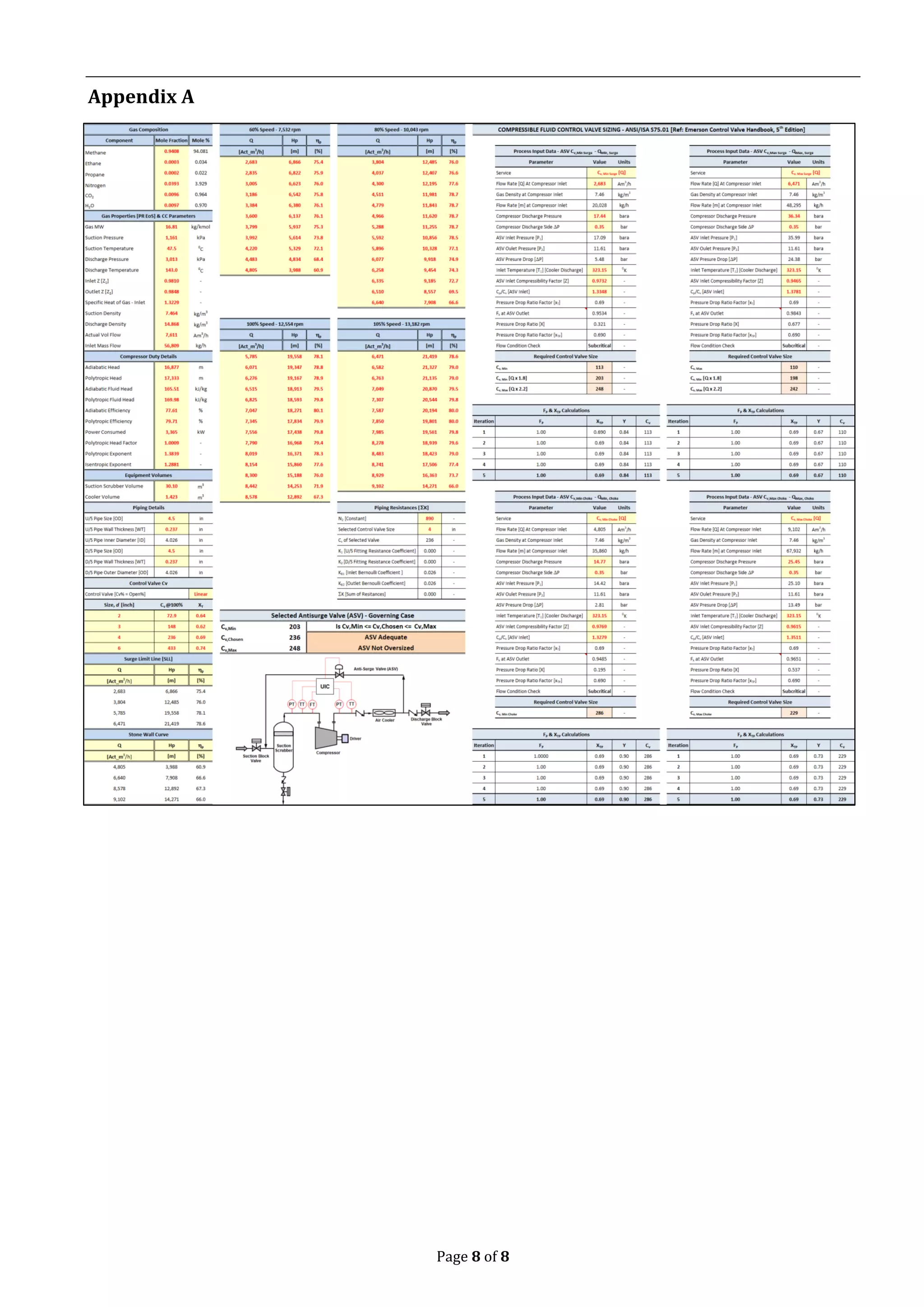
4. Page 4 of 8
Case Study
68.1 MMscfd of hydrocarbon gas at 11.61
bara [suction flange conditions] and 47.470C
is to be compressed to 30.13 bara pressure
[discharge flange conditions]. The
compressed gas is cooled to 500C via an air
cooler. The centrifugal compressor used is a
variable speed configuration. The gas
composition is as follows,
Table 1. Gas Composition
Parameter Mol %
Methane [CH4] 94.09
Ethane [C2H6] 0.03
Propane [C3H8] 0.02
Nitrogen [N2] 3.93
Carbon Dioxide [CO2] 0.96
Water [H2O] 0.97
Total 100
The compressor performance curves for
various operating speeds are as follows,
Figure 3. Compressor Performance Curves
The upstream and downstream piping for the
anti-surge line is taken as NPS 4”, Ref [2] with
a thickness of 0.237 inches for this exercise.
The anti-surge valve chosen to be checked is a
NPS 4” valve [OD 4.5”] [Single ported, Cage
Guided, Globe Style Valve body] with a Cv of
236 and corresponding XT value of 0.69.
The surge control line [SCL] chosen for this
exercise is taken as 10% on the surge flow
rate at each speed and is as follows,
Table 2. Surge Control Line [SCL] Parameters
Speed Surge Flow  10% HP
[rpm] [Act_m3/h] [m]
7,532 2,952 6,721
10,043 4,184 12,297
12,544 6,363 19,263
13,182 7,118 21,077
The Gas Properties are as follows for the
suction and discharge flange conditions,
Table 3. Gas Properties at Flange Conditions
Parameter Value Units
Gas MW 16.81 kg/kmol
Suction Pressure 11.61 bara
Suction Temperature 47.5 0C
Discharge Pressure 30.13 bara
Discharge Temperature 143.0 C
Inlet Z [Z1] 0.9810 -
Outlet Z [Z2] 0.9848 -
Specific Heat of Gas - Inlet 1.3229 -
Suction Density 7.464 kg/m3
Discharge Density 14.868 kg/m3
Actual Volumetric Flow 7,611 Am3/h
Inlet Mass Flow 56,809 kg/h
The compressor parameters are as follows,
Table 4. Compressor Parameters
Parameter Value Units
Adiabatic Head 16,887 m
Polytropic Head 17,333 m
Adiabatic Efficiency 77.61 %
Polytropic Efficiency 79.71 %
Power Consumed 3,365 kW
Polytropic Head Factor 1.0009 -
Polytropic Exponent 1.3839 -
Isentropic Exponent 1.2881 -

5. Page 5 of 8
ASV Sizing Solution
Proceeding with the Cv calculation for the
case of Minimum Speed - Surge Flow [Q1],
𝐾𝐵1 = 1 − (
4
4.026
)
4
= 0.026 (16)
𝐾𝐵2 = 1 − (
4
4.026
)
4
= 0.026 (17)
𝐾1 = 0.5 × [1 − (
42
4.0262
)]
2
= 0.000083 (18)
𝐾2 = 1.0 × [1 − (
42
4.0262
)]
2
= 0.00017 (19)
∑ 𝐾 = 0.000083 + 0.00017 + 0.26 − 0.26 (20)
∑ 𝐾 = 0.00025 (21)
𝐹𝑃 = [1 +
0.00025
890
(
236
42
)
2
]
−1
2⁄
= 1 (22)
The flow rate for the minimum speed - surge
flow is 2,683 Am3/h and gas density at
compressor inlet is,
𝜌𝑠 =
11.61×16.81
0.981×0.0831447×320.62
= 7.464
𝑘𝑔
𝑚3
(23)
𝑀 = 2,683 × 7.464 = 20,028
𝑘𝑔
ℎ
(24)
The compressor discharge flange pressure is
17.44 bara at minimum speed surge flow of
2,683 Am3/h and a discharge air cooler which
offers a pressure drop for the flowing gas.
Taking a max P of 0.35 bar across the
discharge side, the ASV inlet pressure
becomes, 17.44 – 0.35 = 17.09 bara. The
cooler discharge temperature is 500C,
therefore neglecting heat losses; the ASV inlet
temperature also is at 500C.
Making an approximation that the ASV
discharge side piping and suction pressure
drop is negligible; the ASV outlet pressure is
nearly equal to the ASV outlet pressure.
Therefore the ASV inlet pressure becomes
11.61 bara. The ASV P is,
∆𝑃 = 17.09 − 11.61 = 5.48 𝑏𝑎𝑟 (25)
The ASV Inlet Z & k1 value [Cp/Cv] at 17.09
bara and 500C is 0.9732 and 1.3348.
The gas specific heat ratio to air specific heat
ratio is calculated as,
𝐹𝑘 =
1.3348
1.4
= 0.9534 (26)
The pressure drop ratio factor [XT] is,
𝑋 =
5.48
17.09
= 0.321 (27)
Since the valve construction details are
available, XTP is used instead of XT.
𝑋 𝑇𝑃 =
0.69
12
× [1 +
0.69(0+0.026)
1000
(
236
42
)
2
]
−1
(28)
𝑋 𝑇𝑃 = 0.69 (29)
Checking for flow condition,
𝐹𝑘 × 𝑋 𝑇𝑃 = 0.9534 × 0.69 = 0.6579 (30)
Since X < Fk  XTP, flow is Subcritical.
The gas expansion factor is estimated as,
𝑌 = 1 −
0.321
3×0.9534×0.69
= 0.8374 (31)
Therefore the ASV Cv is computed as,
𝐶𝑣 =
20,028
94.8×1×17.09×0.8374√
0.321×16.81
323.15×0.9732
(32)
𝐶𝑣 = 112.721 (33)
Re-inserting the value of Cv = 112.72 into the
Fp expression to iterate, the value of Cv
becomes,
𝐹𝑃 = [1 +
0.00025
890
(
112.721
42
)
2
]
−1
2⁄
= 0.9999 (34)
𝐶𝑣 =
20,028
94.8×0.9999×17.09×0.8375√
0.321×16.81
323.15×0.9732
(35)
𝐶𝑣 = 112.719~113 (36)
Therefore with another iteration the Cv value
remains nearly the same at 112.72 ~ 113.
The ASV Cv can now be estimated for the case
of Q  1.8 at Cv,min and Q  2.2 at Cv,max.
𝐶𝑣,𝑚𝑖𝑛 = 1.8 × 113 = 203 (37)
𝐶𝑣,𝑚𝑎𝑥 = 2.2 × 113 = 248 (38)
Performing similar calculations for all cases,

6. Page 6 of 8
Table 5. ASV Sizing Cases – Surge Points
Parameter
Min
Surge
Max
Surge
Units
Qs 2,683 6,471 Am3/h
s 7.46 7.46 kg/m3
M 20,028 48,295 kg/h
PD 17.44 36 bara
Discharge P 0.35 0.35 bar
ASV Inlet P1 17.09 35.99 bara
ASV Outlet P2 11.61 11.61 bara
ASV P 5.48 24.38 bar
Cooler Outlet T 323.15 323.15 0K
ASV Inlet Z 0.9732 0.9465 -
Cp/Cv-ASV Inlet 1.3348 1.3781 -
XT 0.69 0.69 -
Fk - ASV Outlet 0.9534 0.9843 -
X 0.321 0.677 -
XTP 0.690 0.690 -
Flow Condition Subcritical Subcritical -
Cv, Min 113 110 -
Cv, Min [Q x 1.8] 203 198 -
Cv, Max [Q x 2.2] 248 242 -
Table 6. ASV Sizing Cases – Choke Points
Parameter
Min
Choke
Max
Choke
Units
Qs 4,805 9,102 Am3/h
s 7.46 7.46 kg/m3
M 35,860 67,932 kg/h
PD 14.77 25.45 bara
Discharge P 0.35 0.35 bar
ASV P1 14.42 25.10 bara
ASV P2 11.61 11.61 bara
ASV P 2.81 13.49 bar
Cooler T 323.15 323.15 0K
ASV Inlet Z 0.9769 0.9615 -
Cp/Cv 1.3279 1.3511 -
XT 0.69 0.69 -
Fk 0.9485 0.9651 -
X 0.195 0.537 -
XTP 0.690 0.690 -
Flow Condition Subcritical Subcritical -
Cv, Choke 286 229 -
From the Cv values calculated, the governing
case becomes the Min Speed surge point case.
𝐶𝑣,𝑚𝑖𝑛 = 203 ≤ 𝐶𝑣 = 236 ≤ 𝐶𝑣 = 248 (39)
Hence the selected 4” control valve with a Cv
of 236 and XT of 0.69 is adequately sized to
provide anti-surge control.
Transient Study to Verify ASV Sizing
With the ASV size selected, a transient study
is performed to check for ASV adequacy.
Centrifugal compressors during shutdown
experience surging & the ASV must be able to
provide sufficient cold recycle flow to keep
the operating point away from the SLL as the
compressor coasts down.
Normal shutdown [NSD] refers to a planned
event where the anti-surge valve is opened
first by 100%, prior to a compressor trip.
An emergency shutdown [ESD] is an
unplanned event, where for example, upon
loss of driver power, the ASV opens quickly to
recycle flow and prevent the operating point
from crossing the SLL during coast down. For
this tutorial, the ESD case considered is
“Driver trip” where the compressor driver
experiences a sudden loss of power.
To simulate the transient case, the air cooler
and suction scrubber can be sized with
preliminary estimates to cater to maximum
speed choke flow case.
Suction Scrubber Volume
Using GPSA K-Value method for suction
scrubber sizing, Ref [3], for a flow rate of
67,932 kg/h and 11.61 bara operating

7. Page 7 of 8
pressure, the suction scrubber size is H  D of
6.9m  2.3m with an ellipsoidal head and
inside dish depth of 0.25m. The total scrubber
volume is 30.1 m3.
Air Cooler Volume
Similarly, the air cooler is sized for maximum
speed choke flow case, Ref [4], for a flow rate
of 67,932 kg/h & duty of 4,351 kW. The
overall heat transfer coefficient [U] is
assumed to be 25 W/m2.K. The inlet
temperature is 1420C which is cooled to 500C
with an air side temperature of 350C. The air
cooler geometry chosen for this exercise is a
single tube pass with 3 tube rows & each tube
is 9.144m in length. The fan & motor
efficiencies are taken as 75% and 95%
respectively. With this data, the air cooler has
a tube OD of 1” [0.0254m] & total number of
tubes of 307 [Tube volume of 1.423 m3].
Compressor Coast down
Coast down time is influenced by a number of
factors including fluid resistance, dynamic
imbalance, misalignment between shafts,
leakage and improper lubrication, skewed
bearings, radial or axial rubbing, temperature
effects, transfer of system stresses, resonance
effect to name a few and therefore in reality,
shutdown times can be lower than estimated
by the method shown below.
The decay rate of driver speed is governed by
the inertia of the system consisting of the
compressor, coupling, gearbox & driver,
which are counteracted by the torque
transferred to the fluid. Neglecting the
mechanical losses, the compressor speed
decay rate can be estimated as,
𝑁[𝑡] =
1
1
𝑁 𝑜
+
216,000×𝑘×[𝑡−𝑡 𝑜]
[2𝜋]2×𝐽
(42)
Where, ‘N0’ is the compressor speed before
ESD, ‘J’ is the total system inertia & ‘t0’ is time
at which the ESD is initiated. For this exercise
the total system inertia is taken as 108 kg.m2.
The coast down speed calculated is,
Figure 4. Compressor Coast down Time
From the curve, the compressor is expected
to reach a standstill in ~124 sec.
ESD and NSD Analysis
With the equipment volumes, ASV Cv chosen
and compressor speed decay rate imposed, an
ESD and NSD analyses is performed to track
operating point during coast down.
Figure 5. ESD/NSD Operating Point Migration
From the analysis made, it is seen that the
selected ASV size of 4” [Cv 236] is sufficient to
prevent a surge during ESD and NSD.
References
1. “Development and Design of Antisurge and
Performance Control Systems for
Centrifugal Compressors”, Mirsky S.,
McWhirter J., Jacobson W., Zaghloul M.,
Tiscornia D., 3rd M.E Turbomachinery
Symposium, Feb 2015
2. Control Valve Handbook, Emerson, 5th Ed.
3. https://checalc.com/calc/vertsep.html
4. https://checalc.com/calc/AirExch.html
5. https://www.slideshare.net/VijaySarathy7
/centrifugal-compressor-settle-out-
conditions-tutorial

8. Page 8 of 8
Appendix A