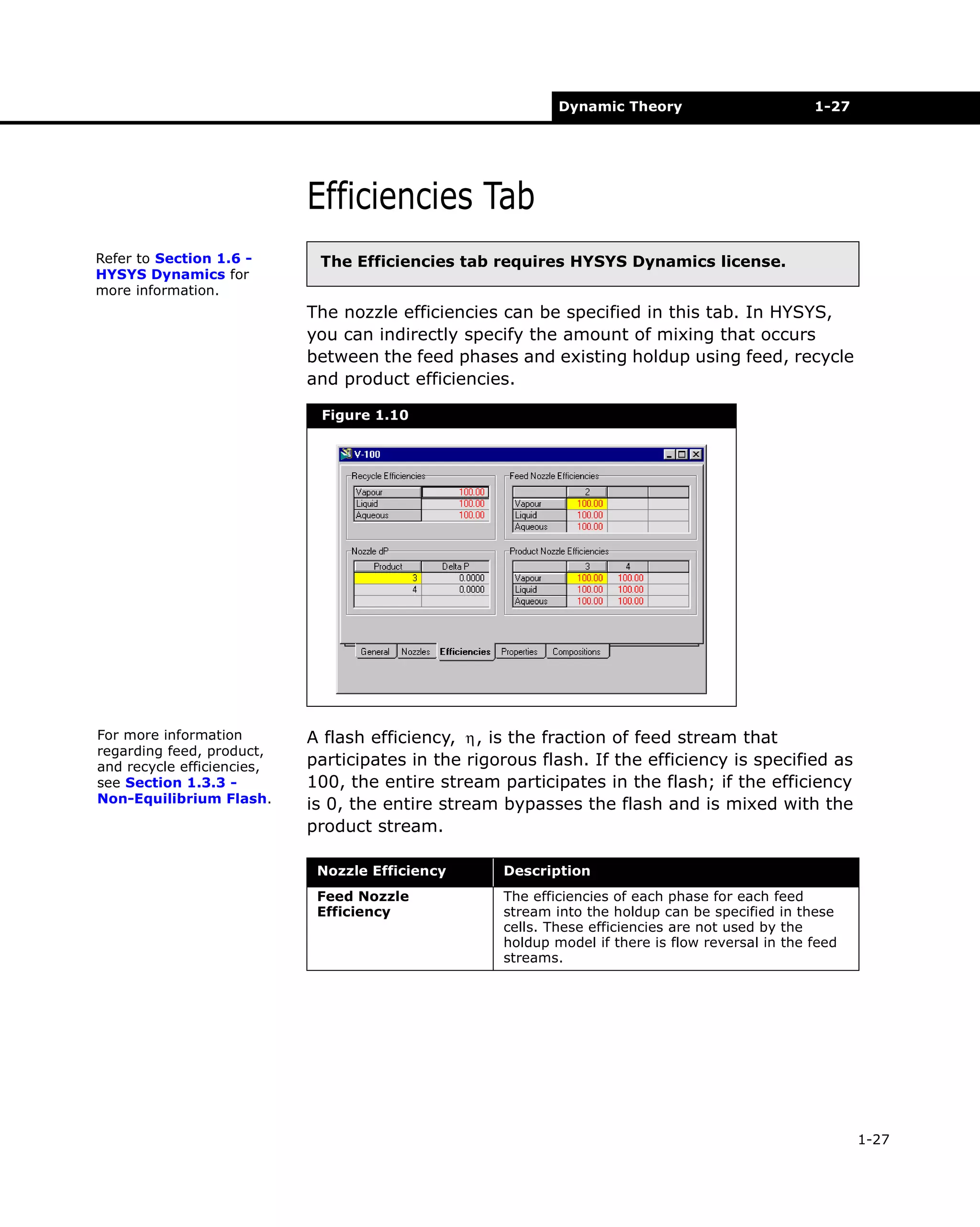
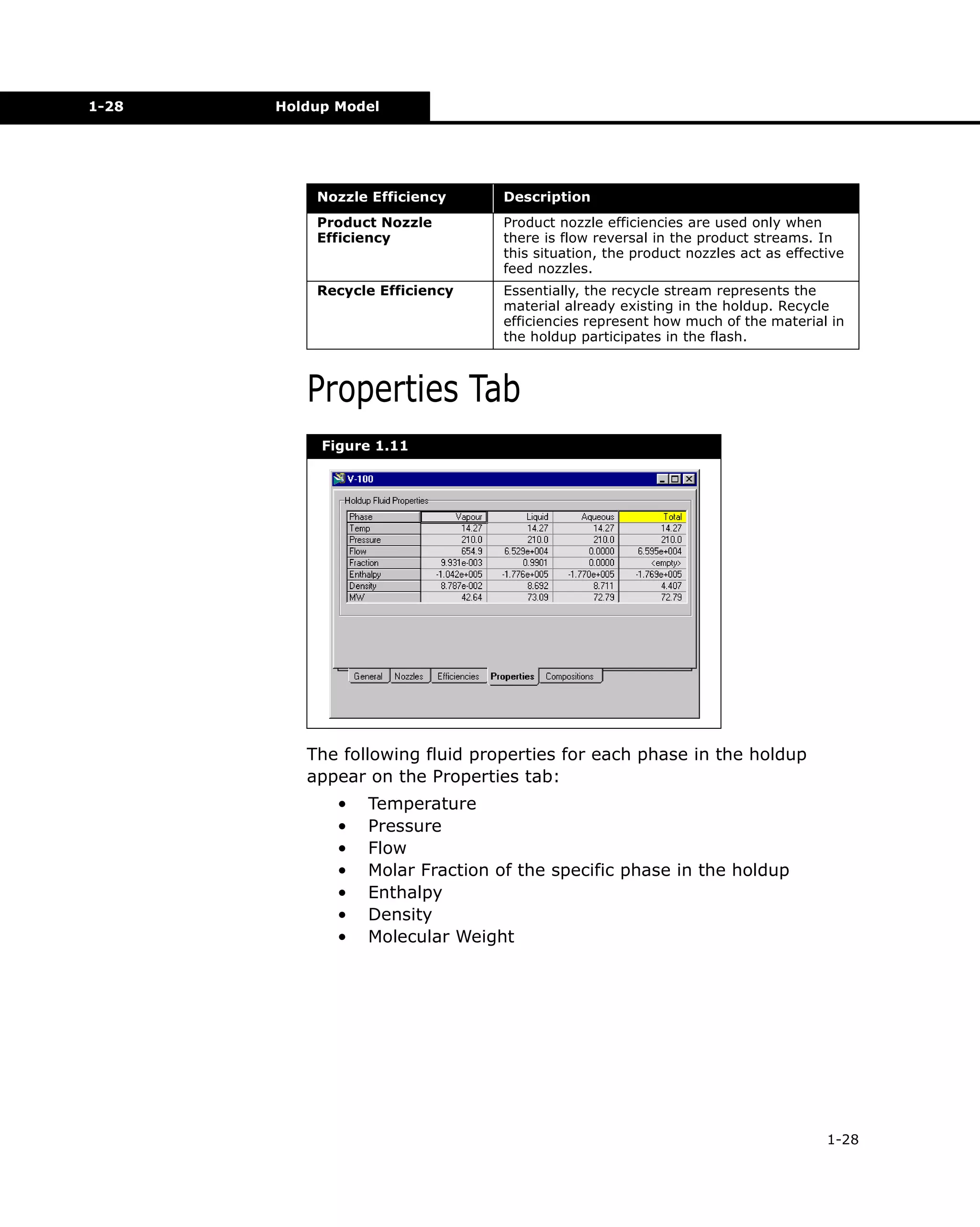
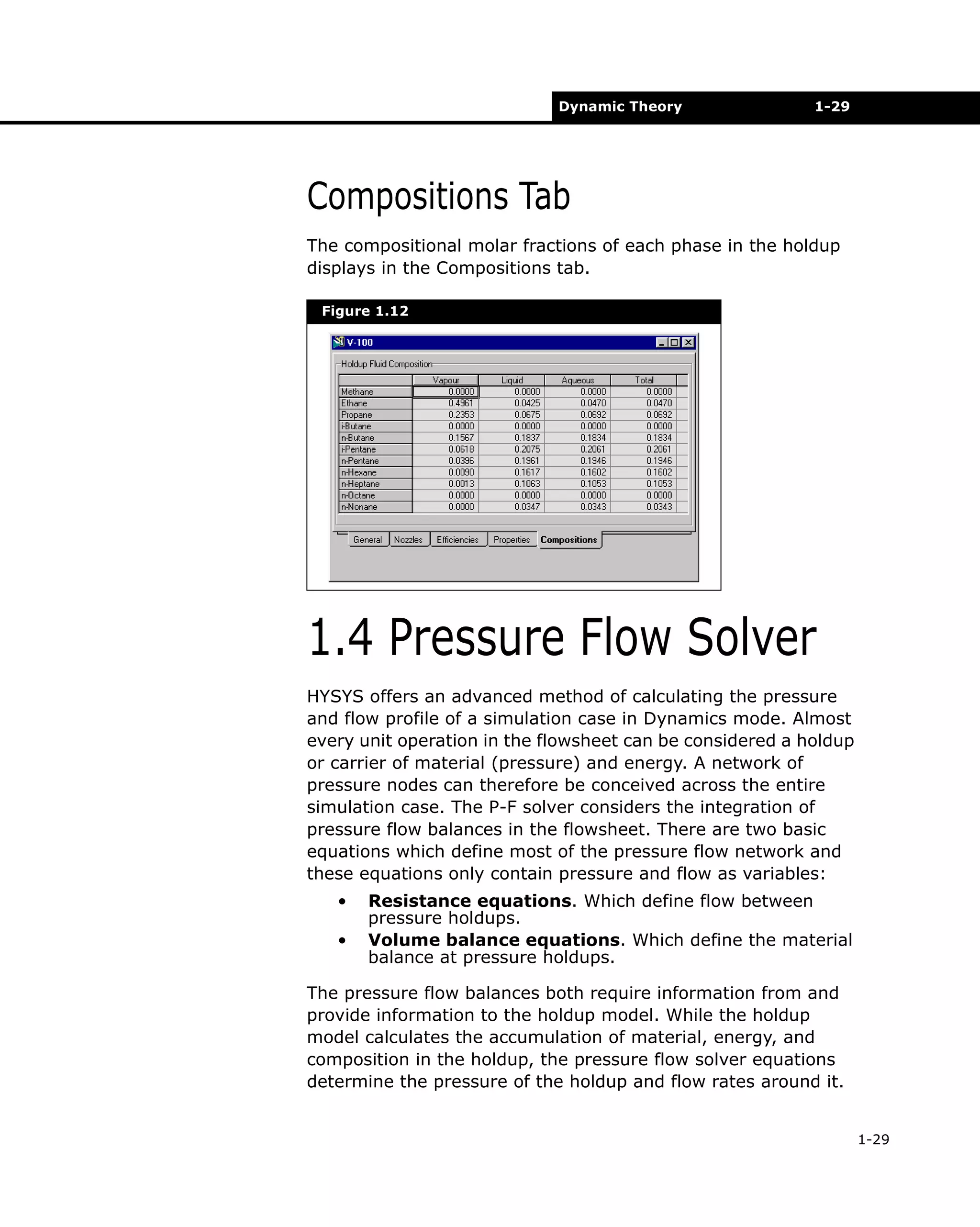
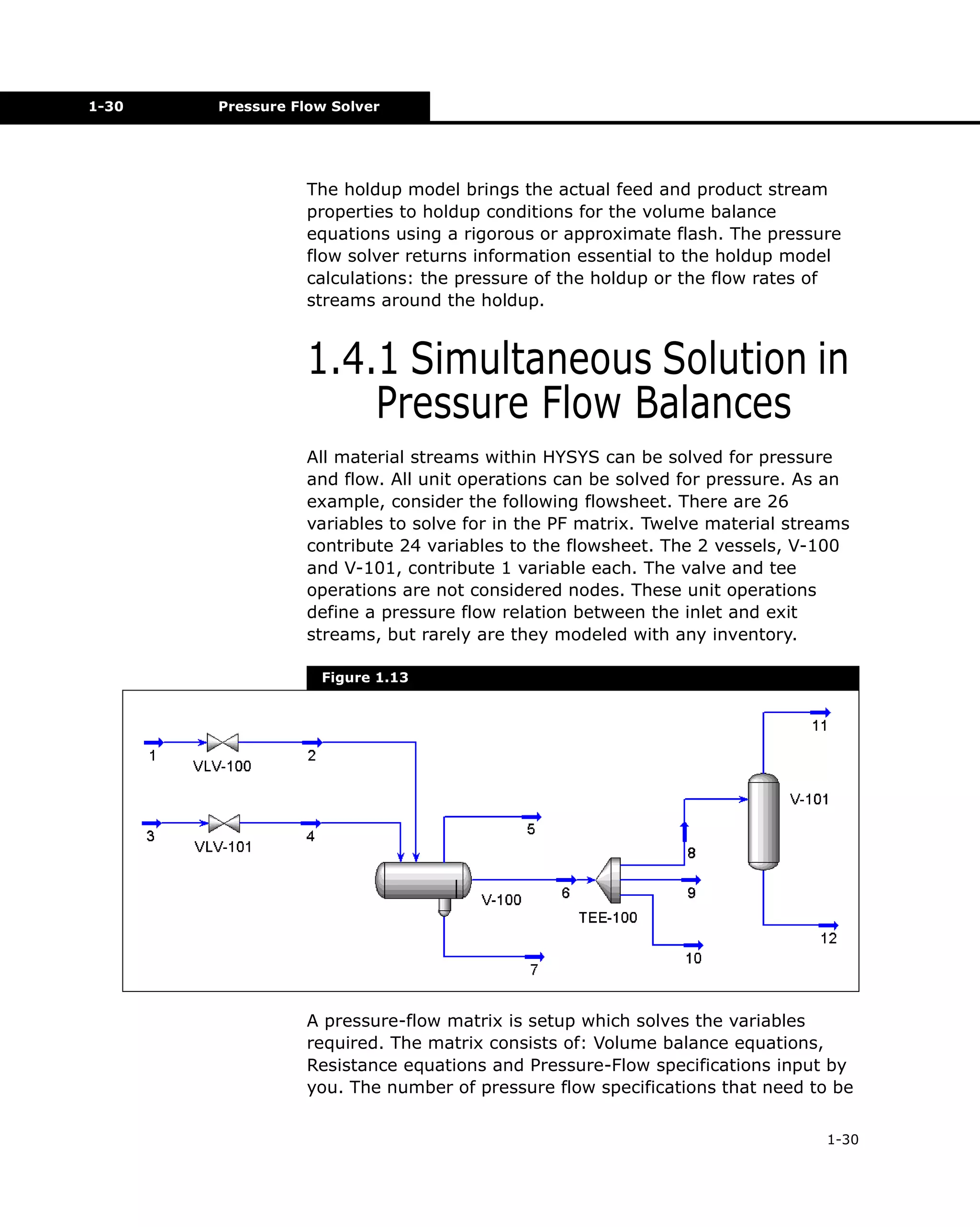
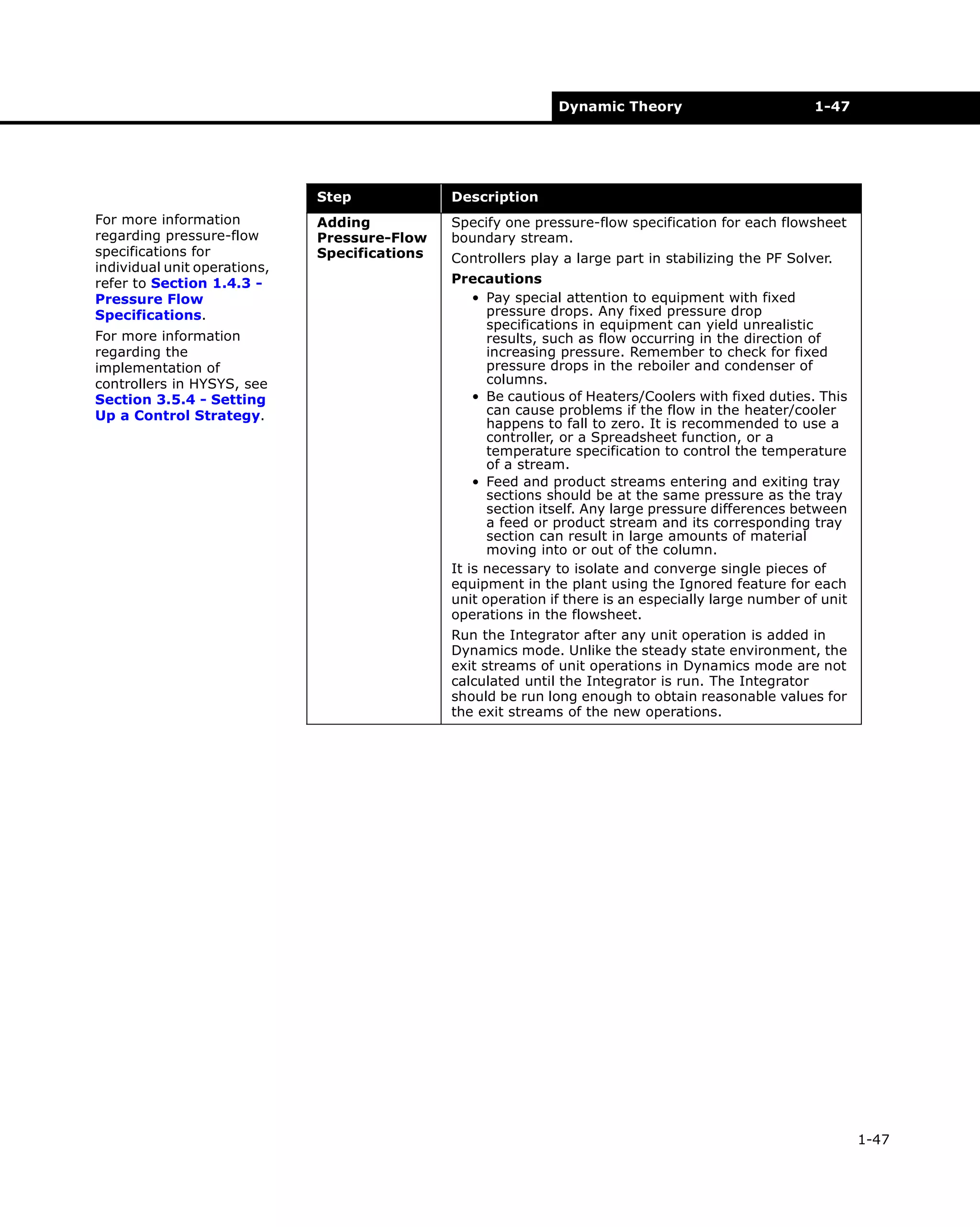
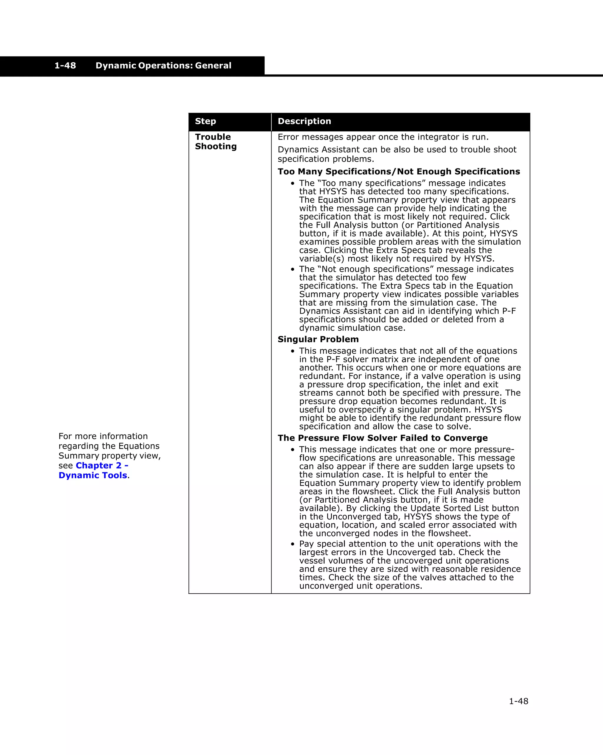
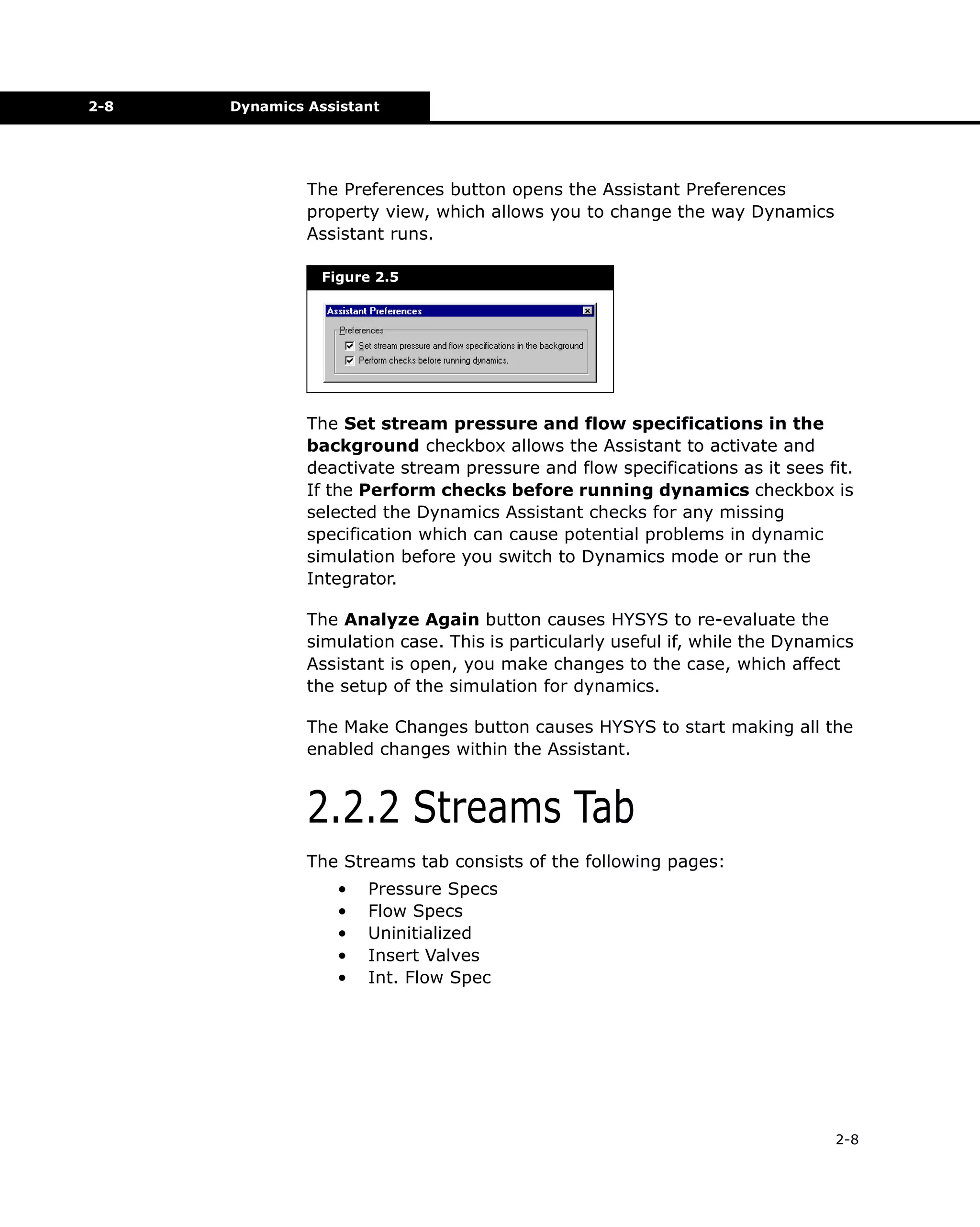
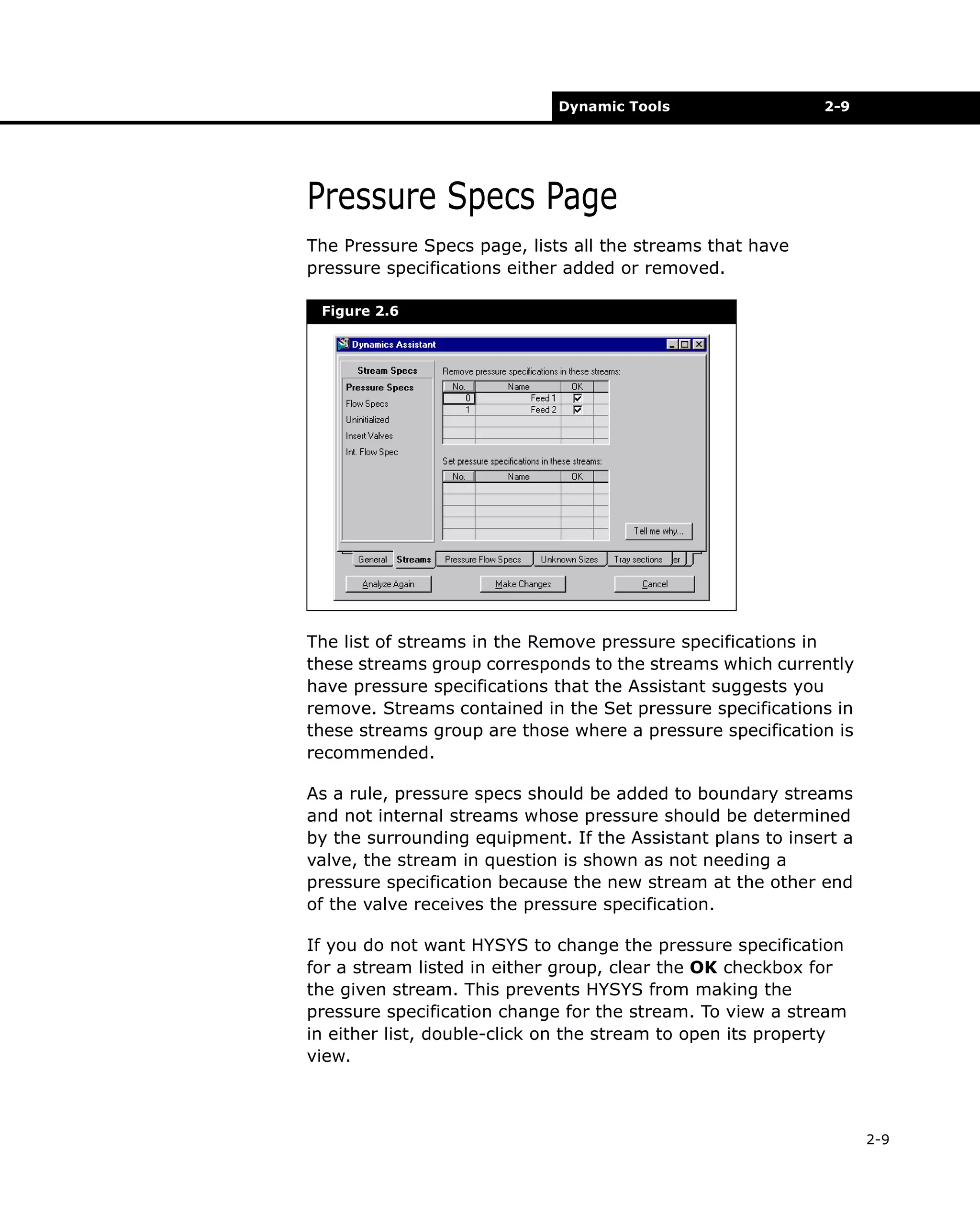
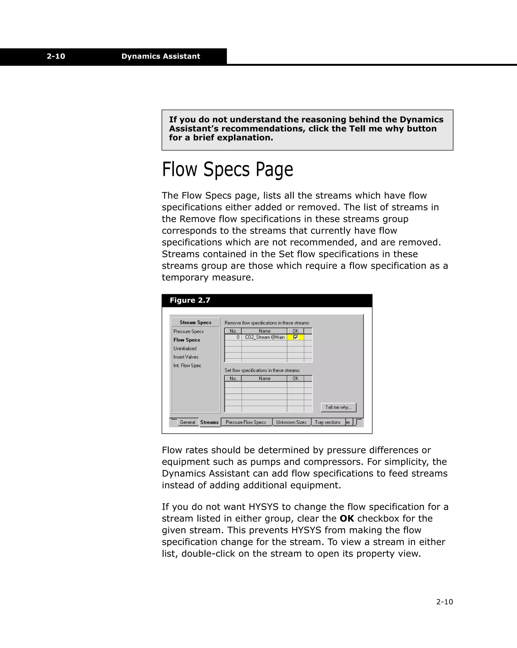
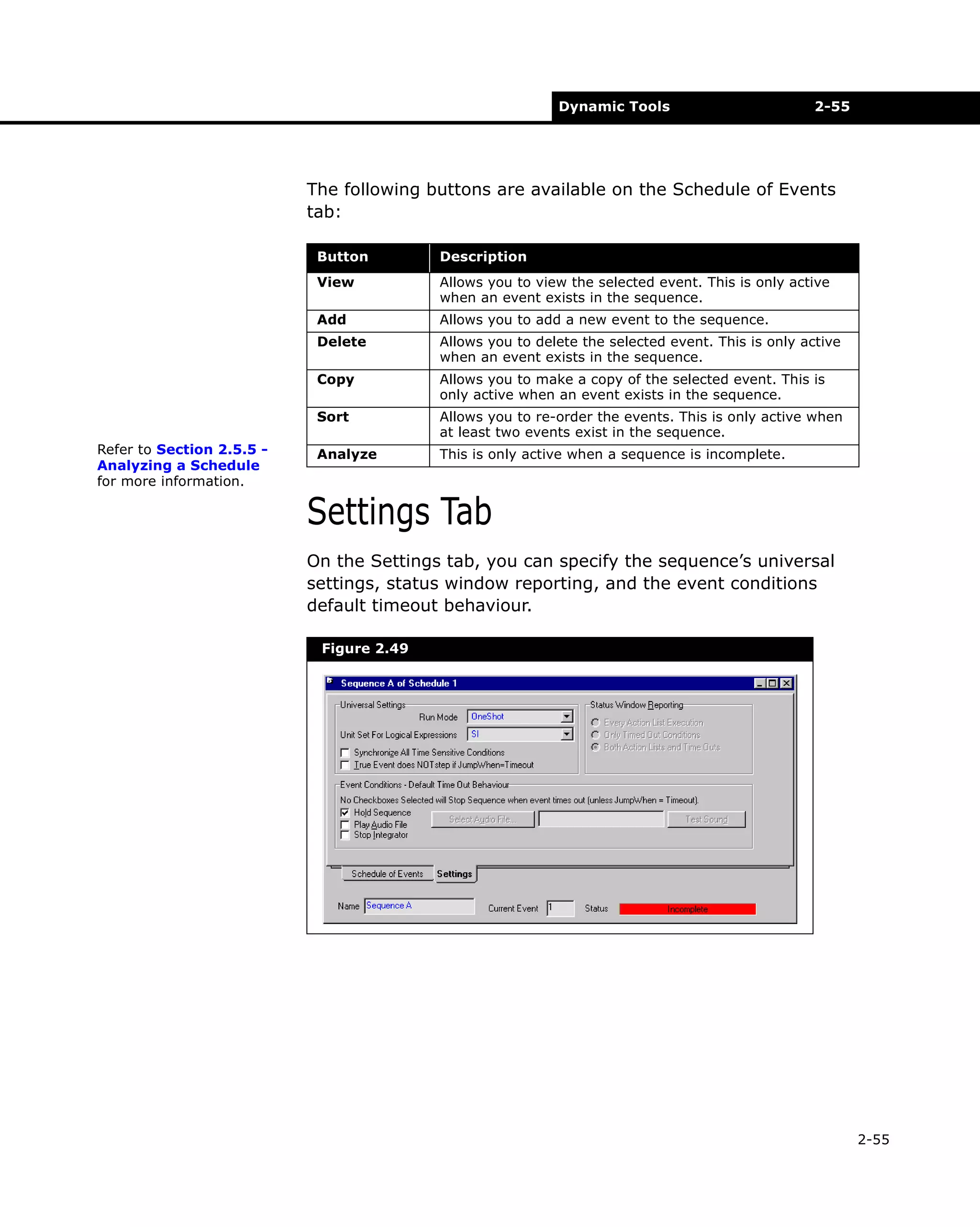
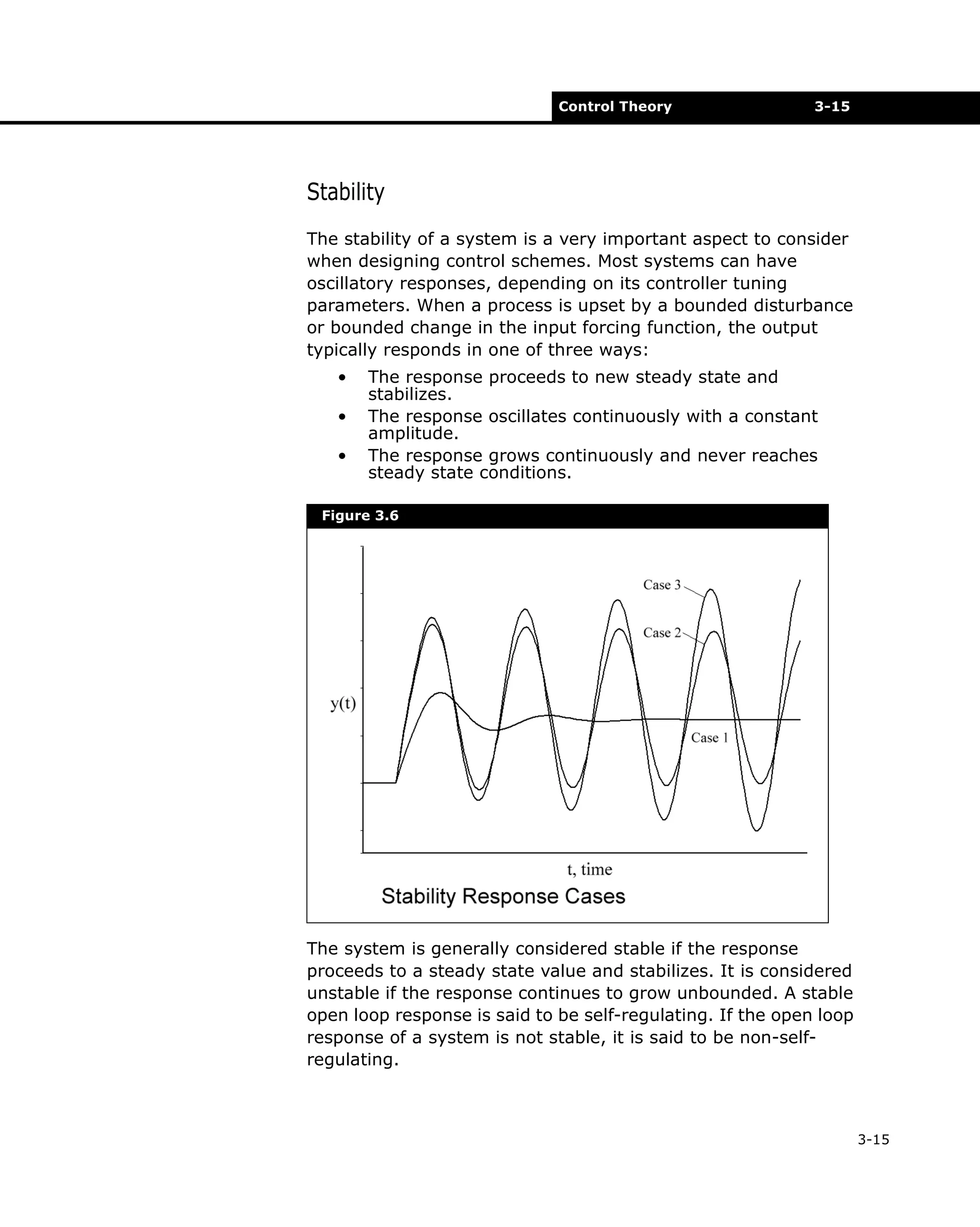
This document provides copyright information and technical support contact details for Aspen Technology's HYSYS 2004.2 Dynamic Modeling software. It lists over 200 Aspen product names that are copyrighted and/or trademarked by Aspen Technology. Contact information is provided for Aspen's Online Technical Support Center, phone support, and email support.


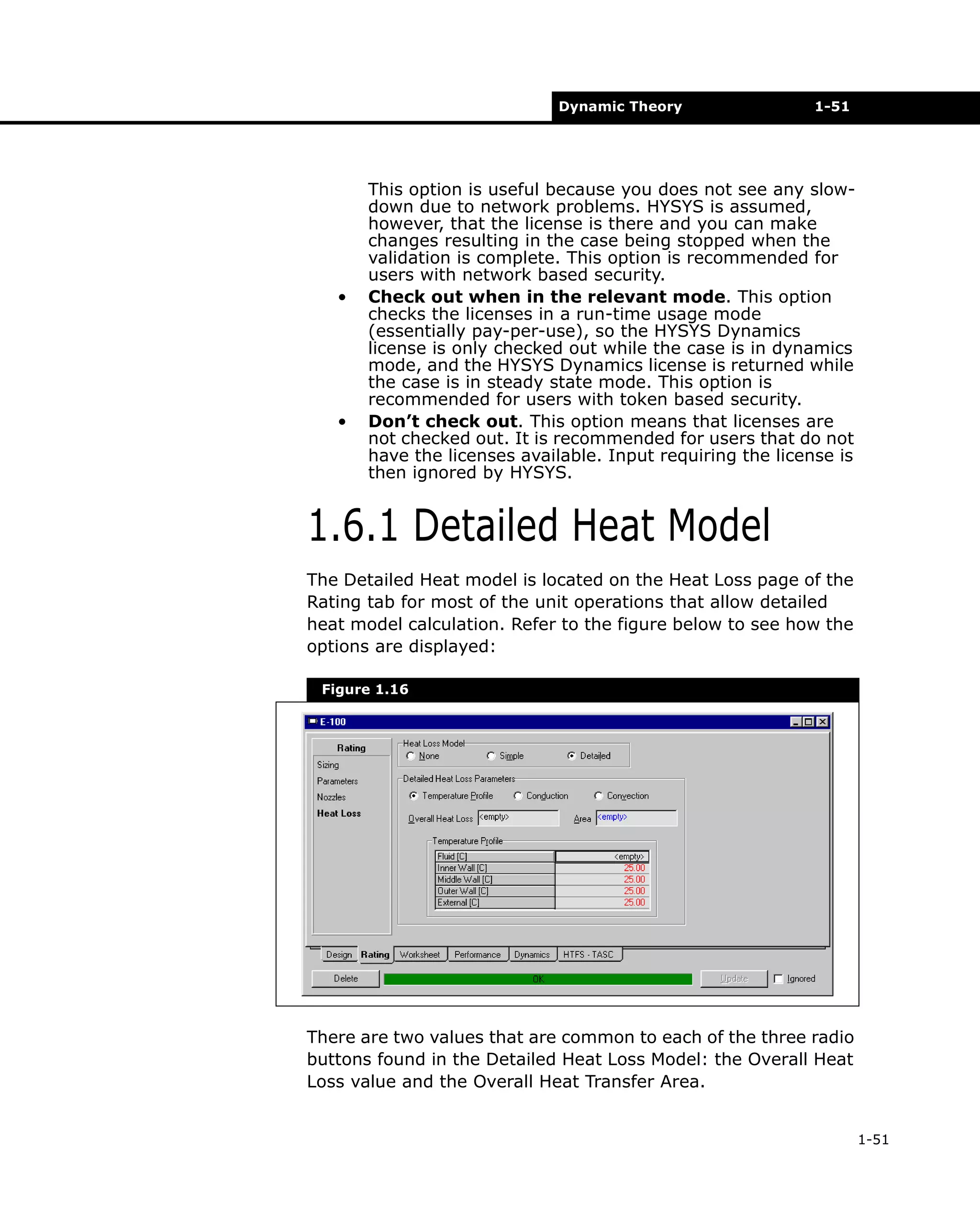
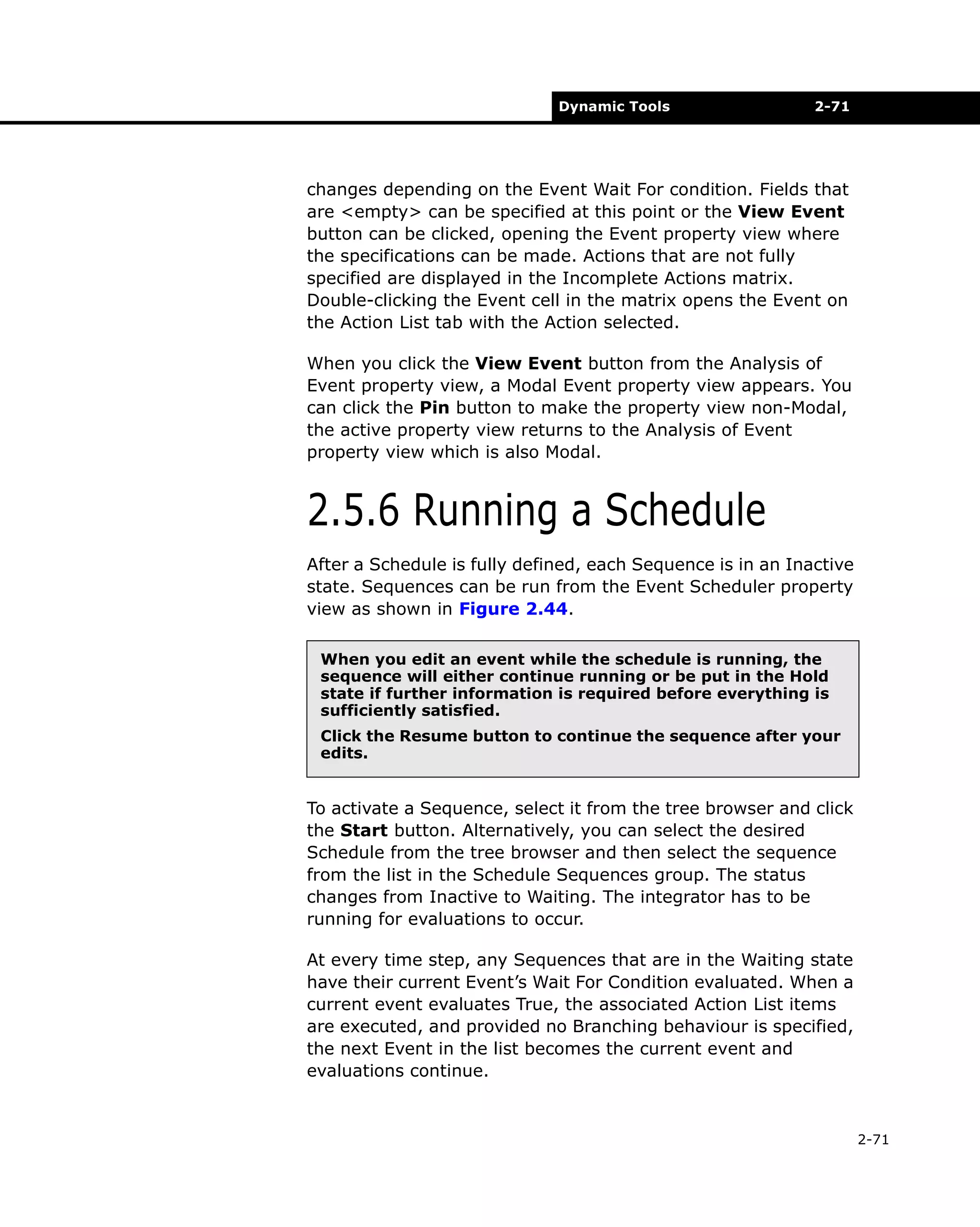
![1-10
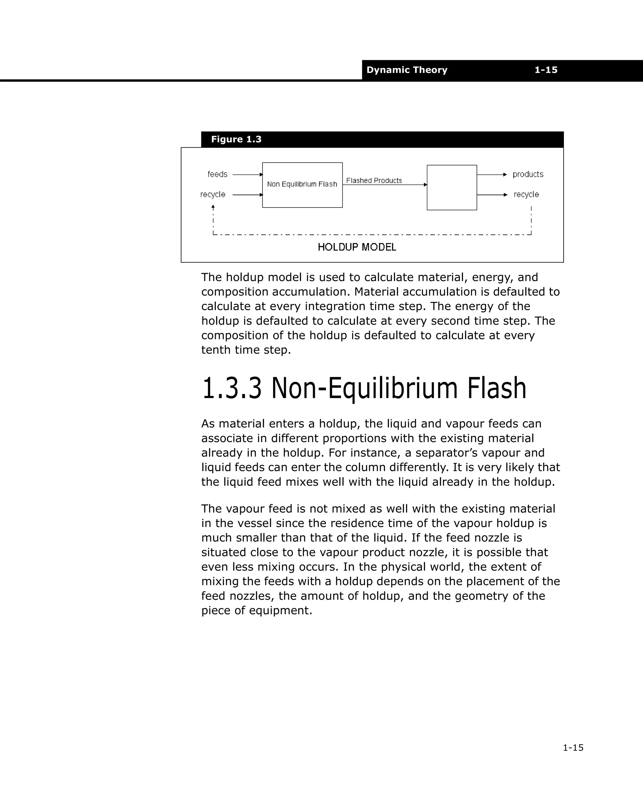
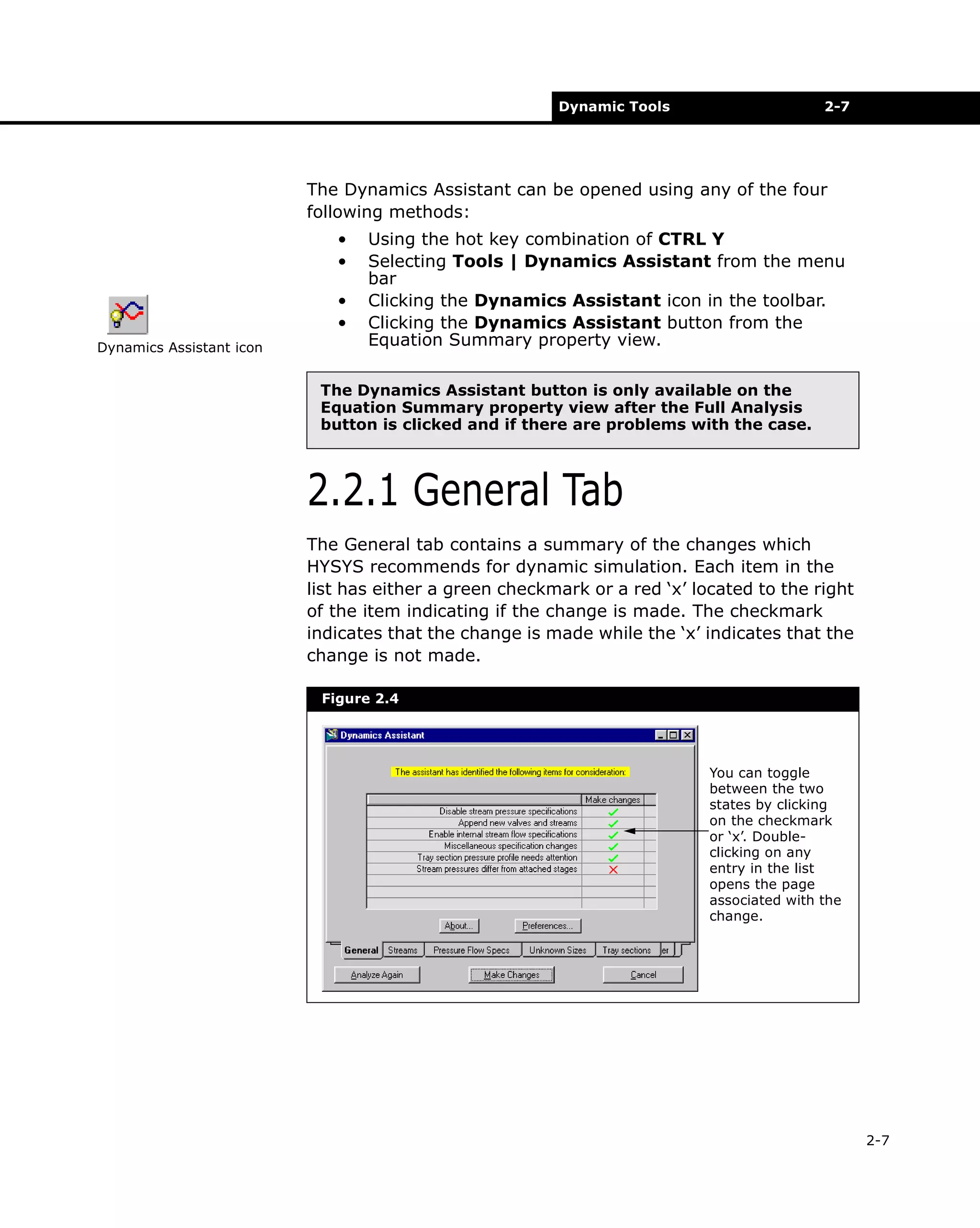
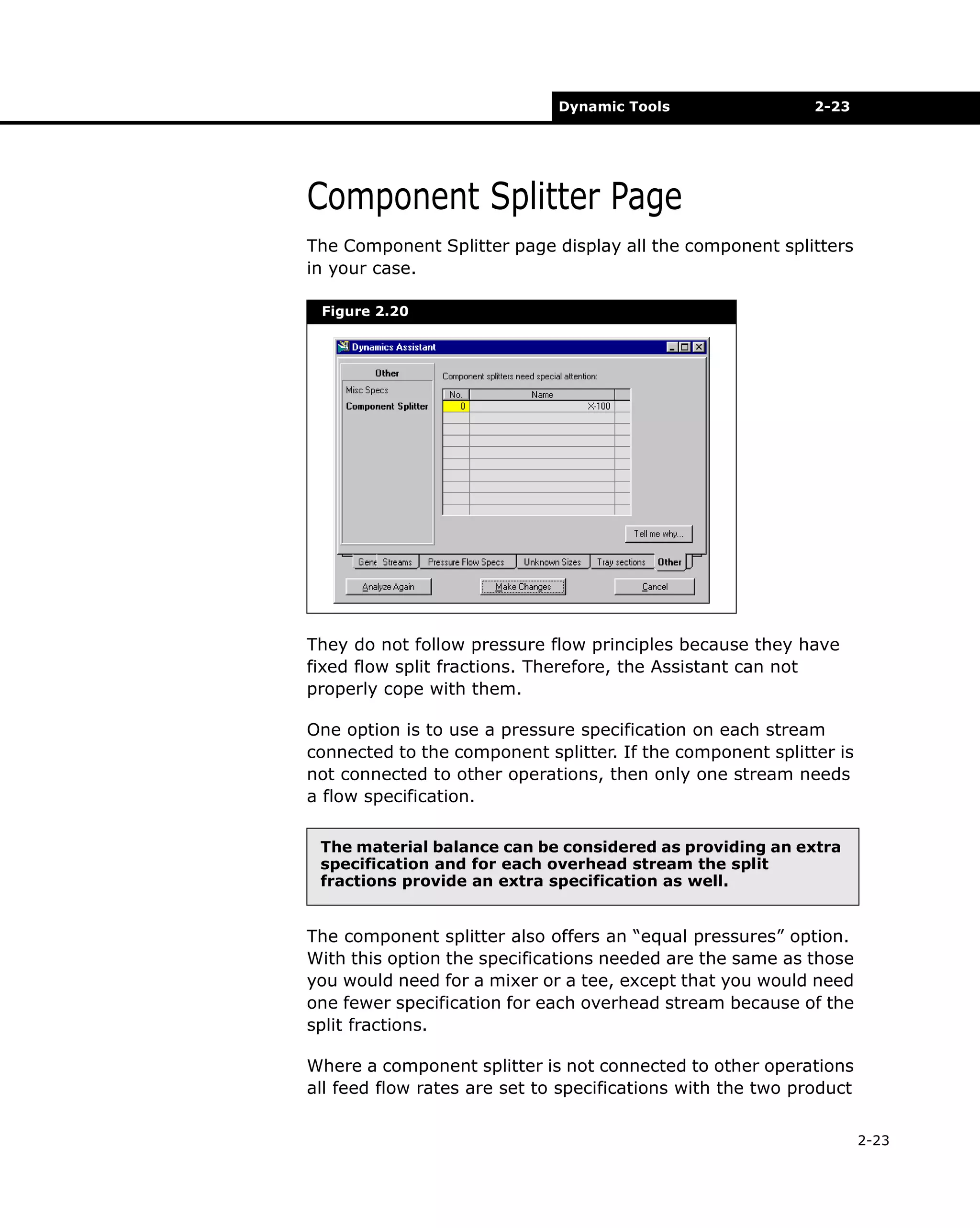
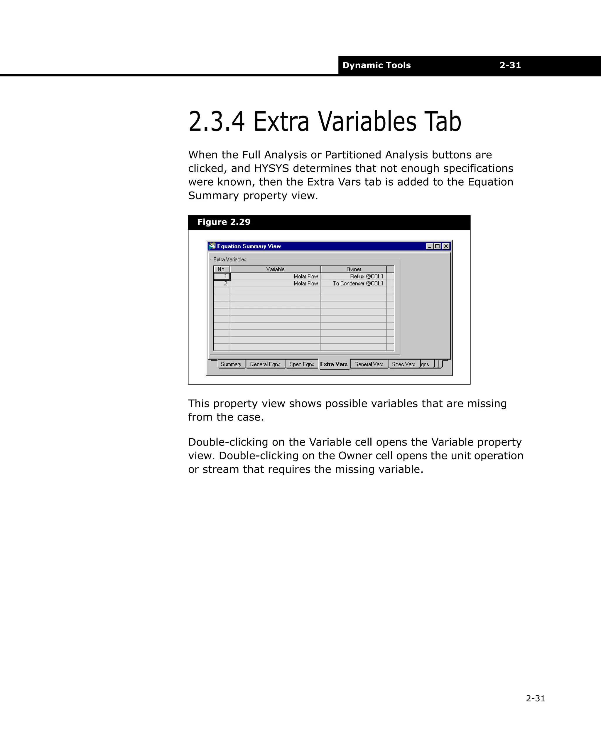
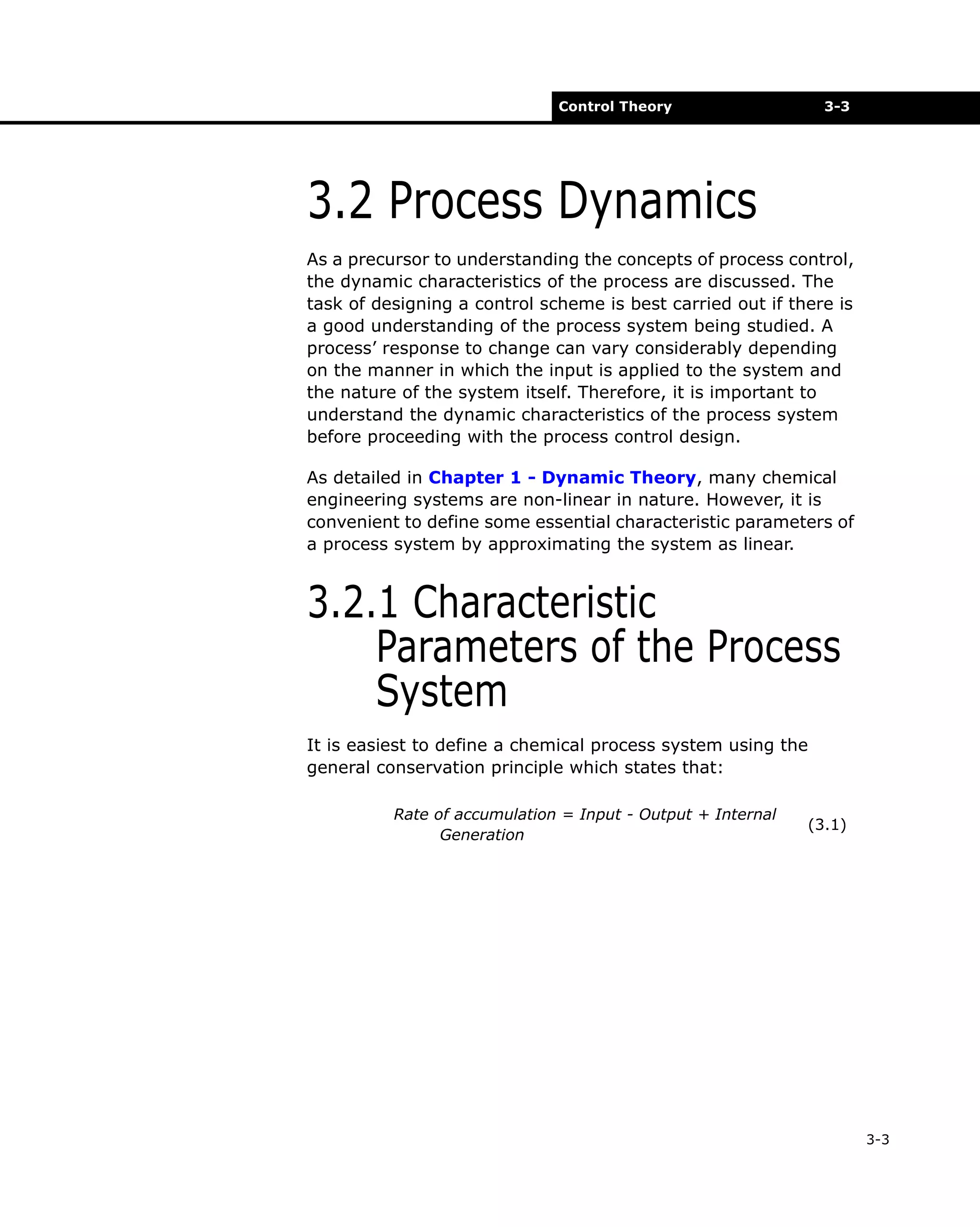
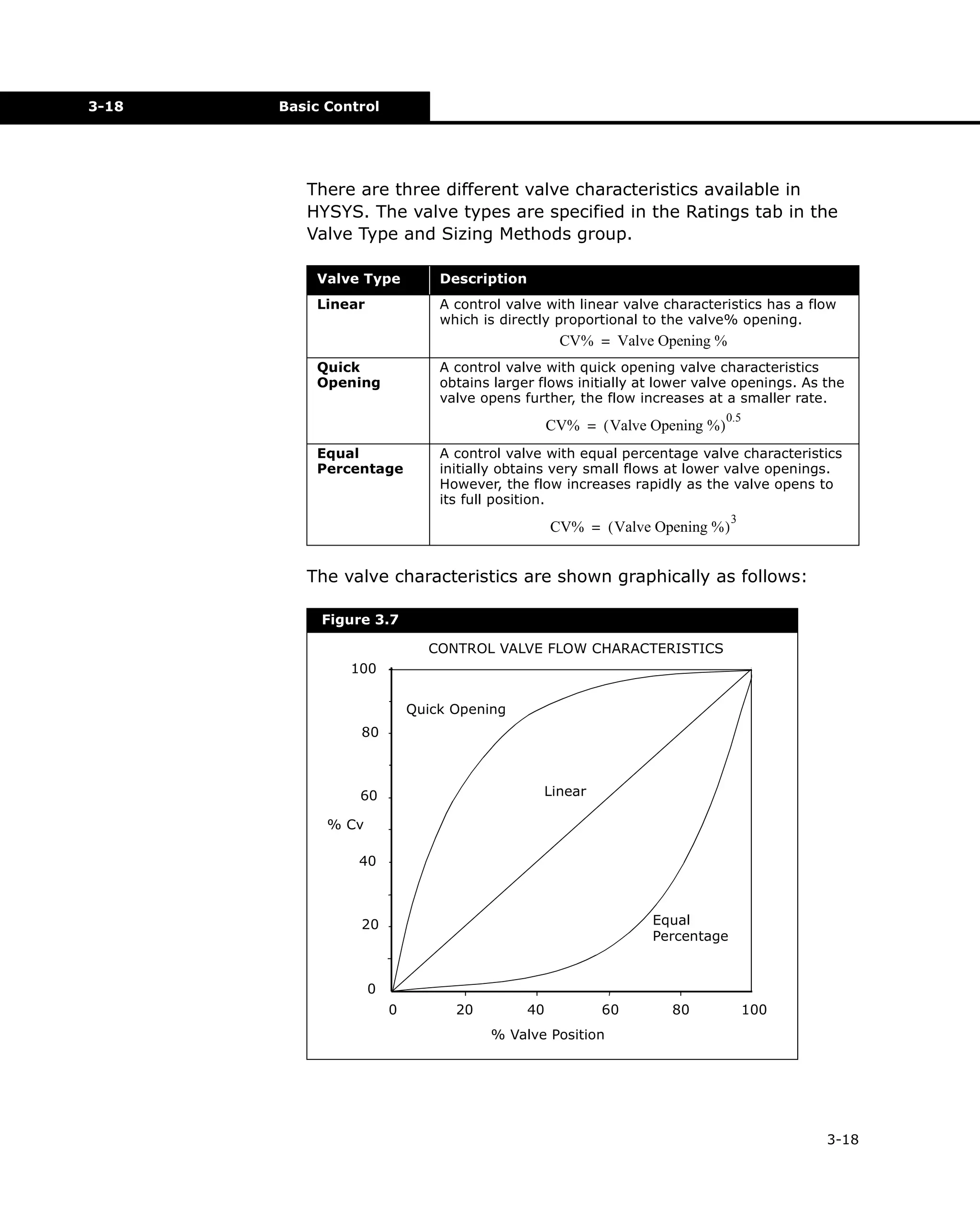
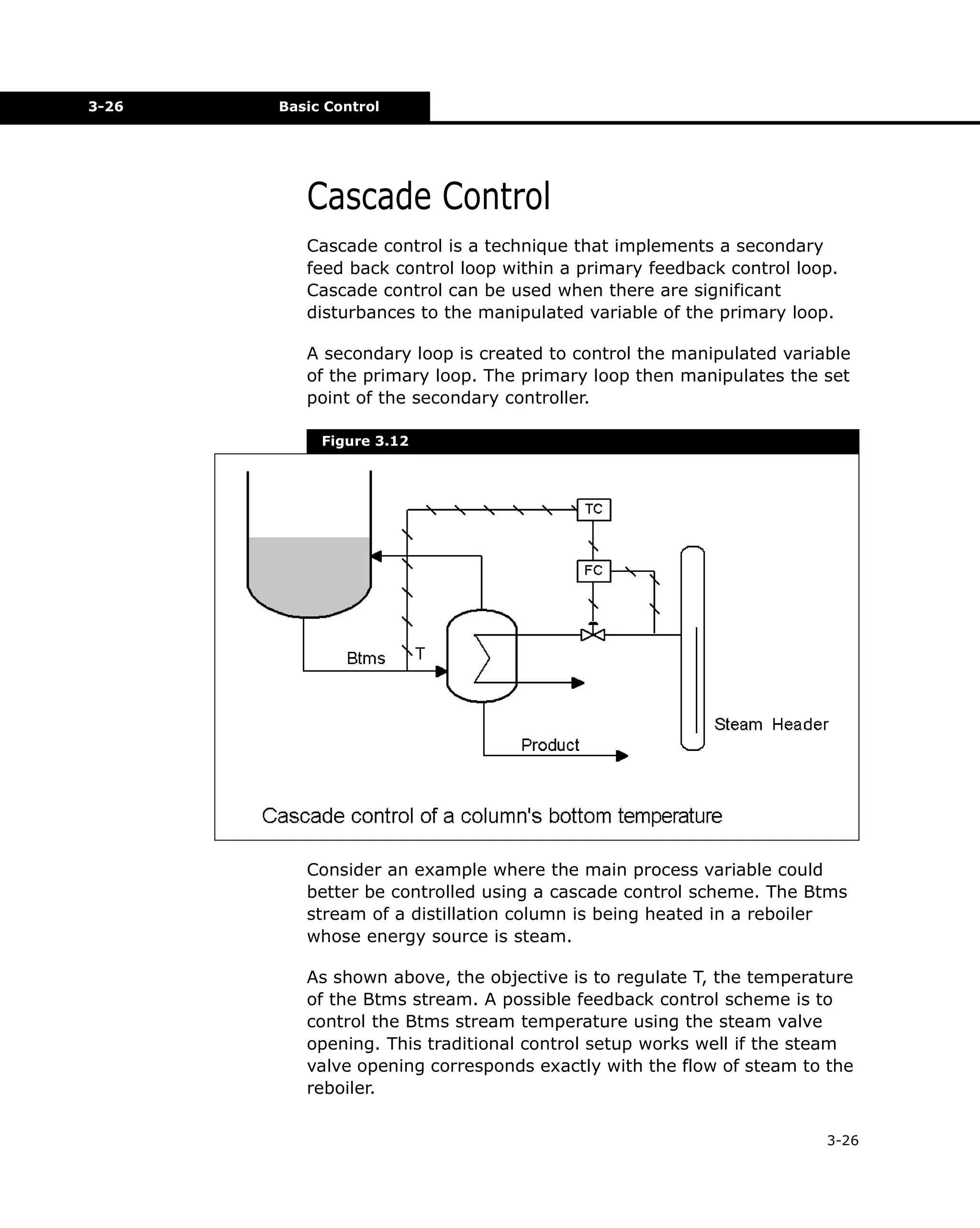
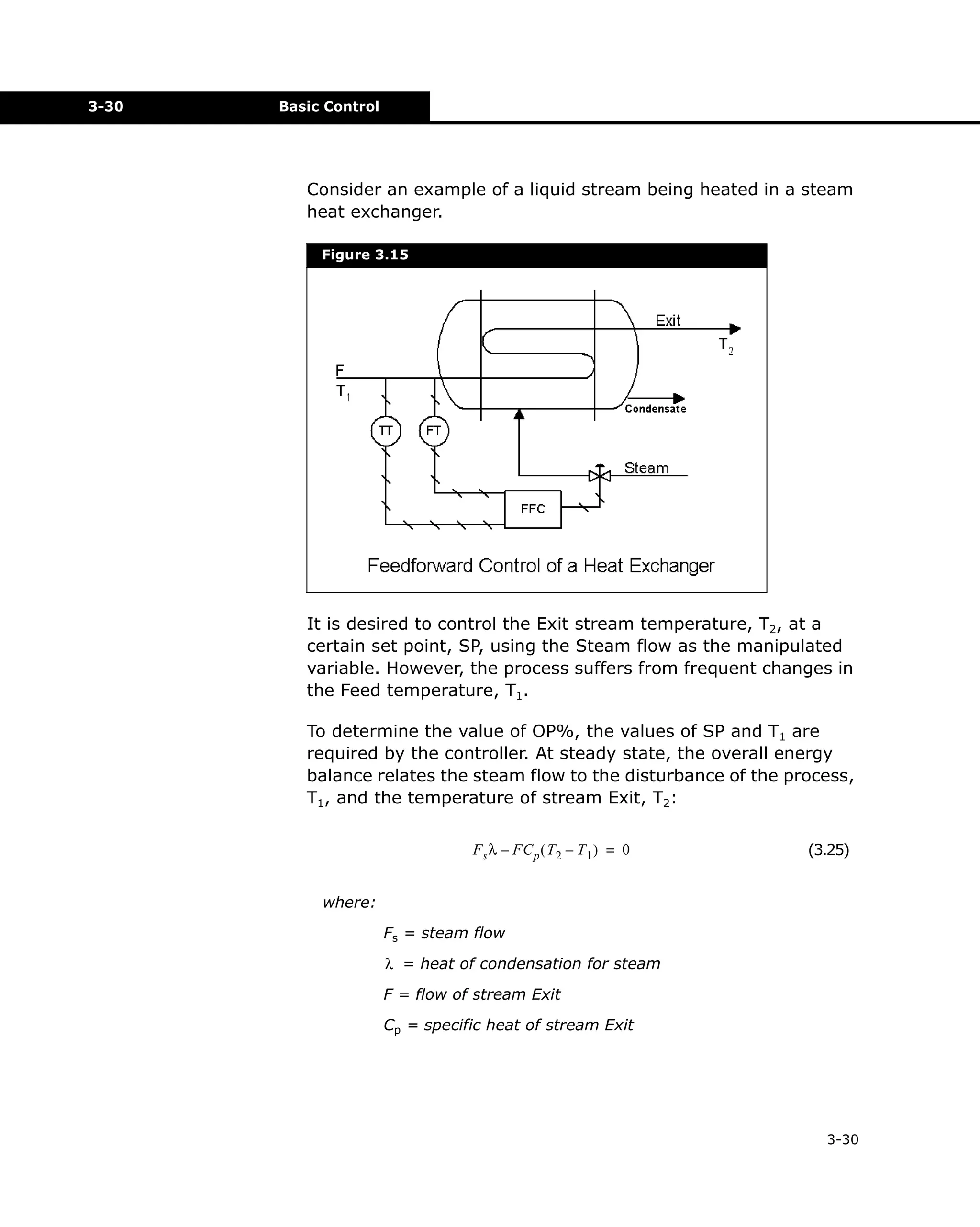
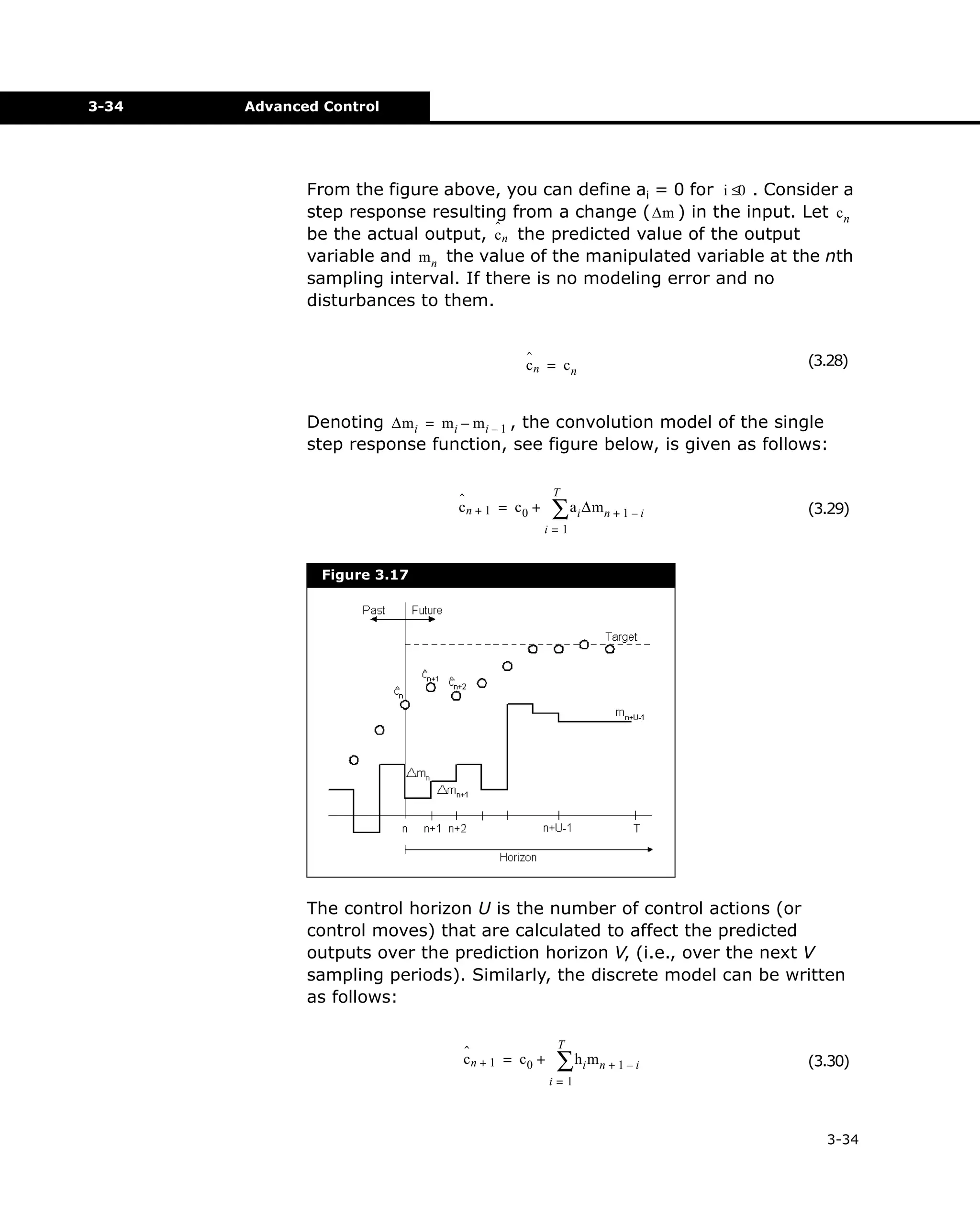
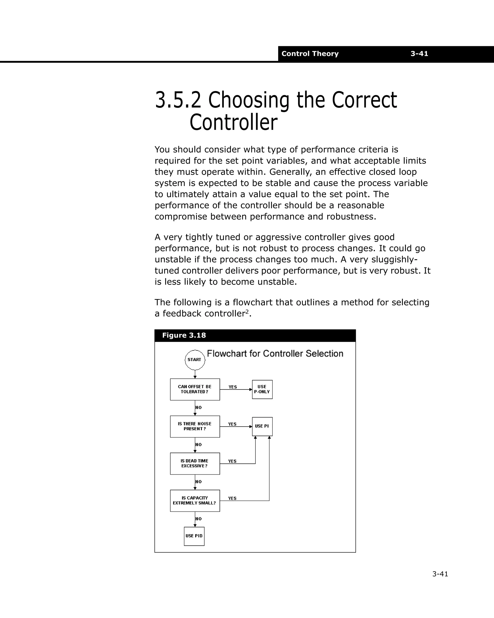
General Concepts
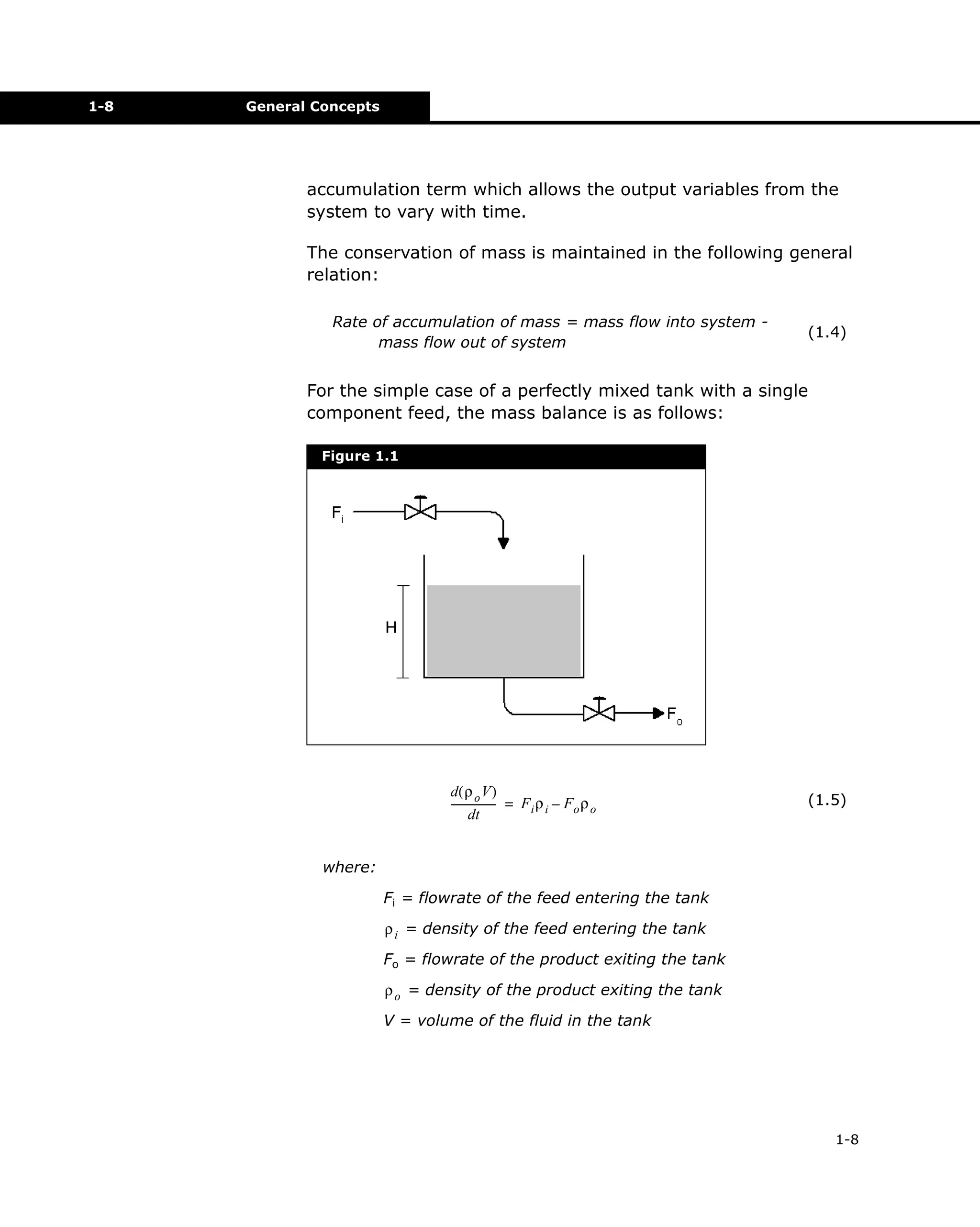
Energy Balance
The energy balance is as follows:
Rate of accumulation of total energy = Flow of total energy
into system - Flow of total energy out of system +
Heat added to system across its boundary + Heat
generated by reaction - Work done by system on
surroundings
(1.8)
The flow of energy into or out of the system is by convection or
conduction. Heat added to the system across its boundary is by
conduction or radiation.
For a CSTR with heat removal, the following general equation
applies:
d [ ( u + k + φ)V ] = F ρ ( u + k + φ ) – F ρ ( u + k + φ ) + Q + Q – ( w + F P – F P )
i i i
i
i
o o o
o
o
r
o o
i i
dt
(1.9)
where:
u = internal energy (energy per unit mass)
k = kinetic energy (energy per unit mass)
φ = potential energy (energy per unit mass)
V = volume of the fluid
w = shaft work done by system (energy per time)
Po = vessel pressure
Pi = pressure of feed stream
Q = heat added across boundary
Qr = DHrxn r A , heat generated by reaction
Several simplifying assumptions can usually be made:
•
•
•
The potential energy can almost always be ignored; the
inlet and outlet elevations are roughly equal.
The inlet and outlet velocities are not high, therefore
kinetic energy terms are negligible.
If there is no shaft work (no pump), w=0.
1-10](https://image.slidesharecdn.com/aspenhysysdynamicmodeling-140221173504-phpapp02/75/Aspen-hysys-dynamic-modeling-17-2048.jpg)
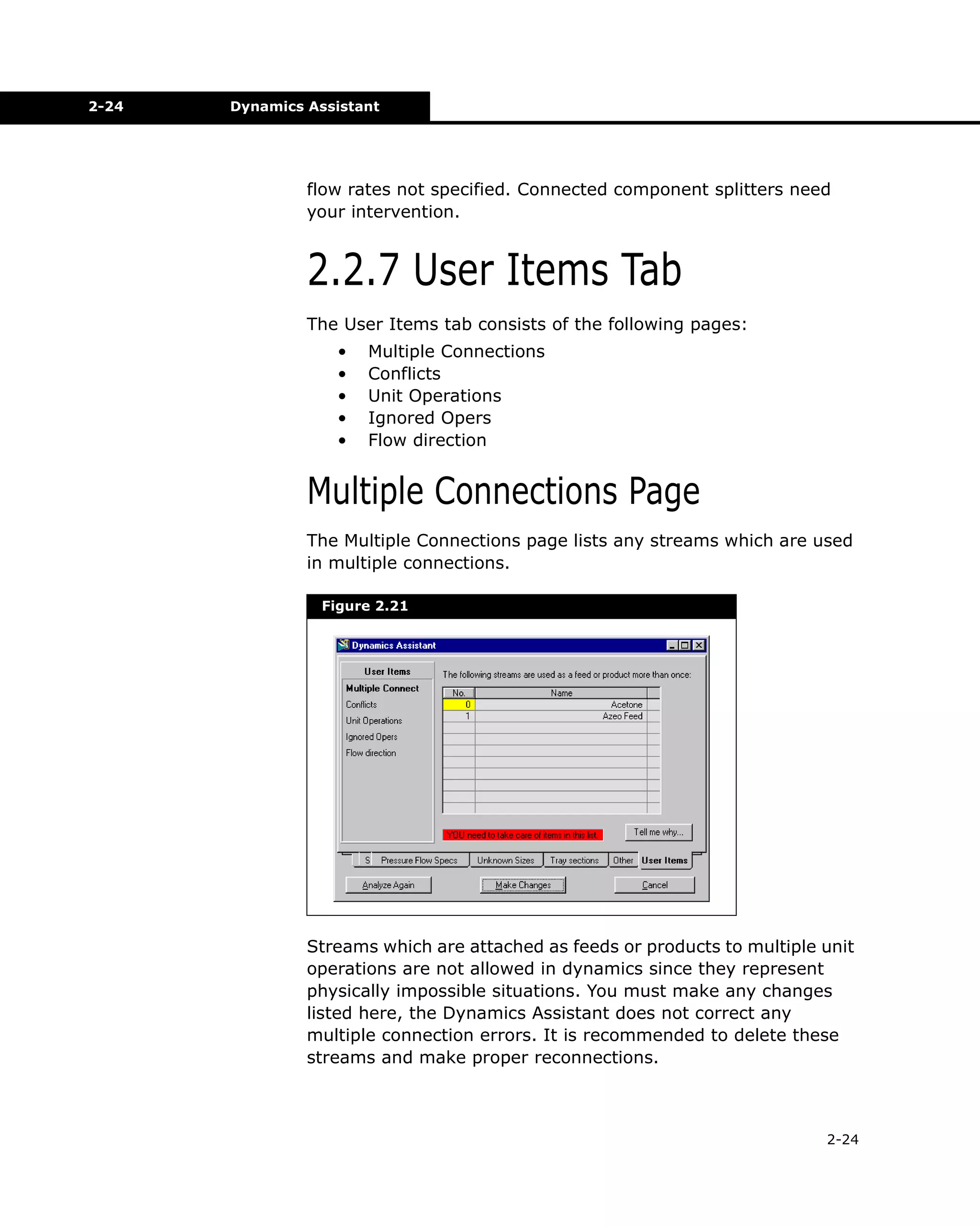
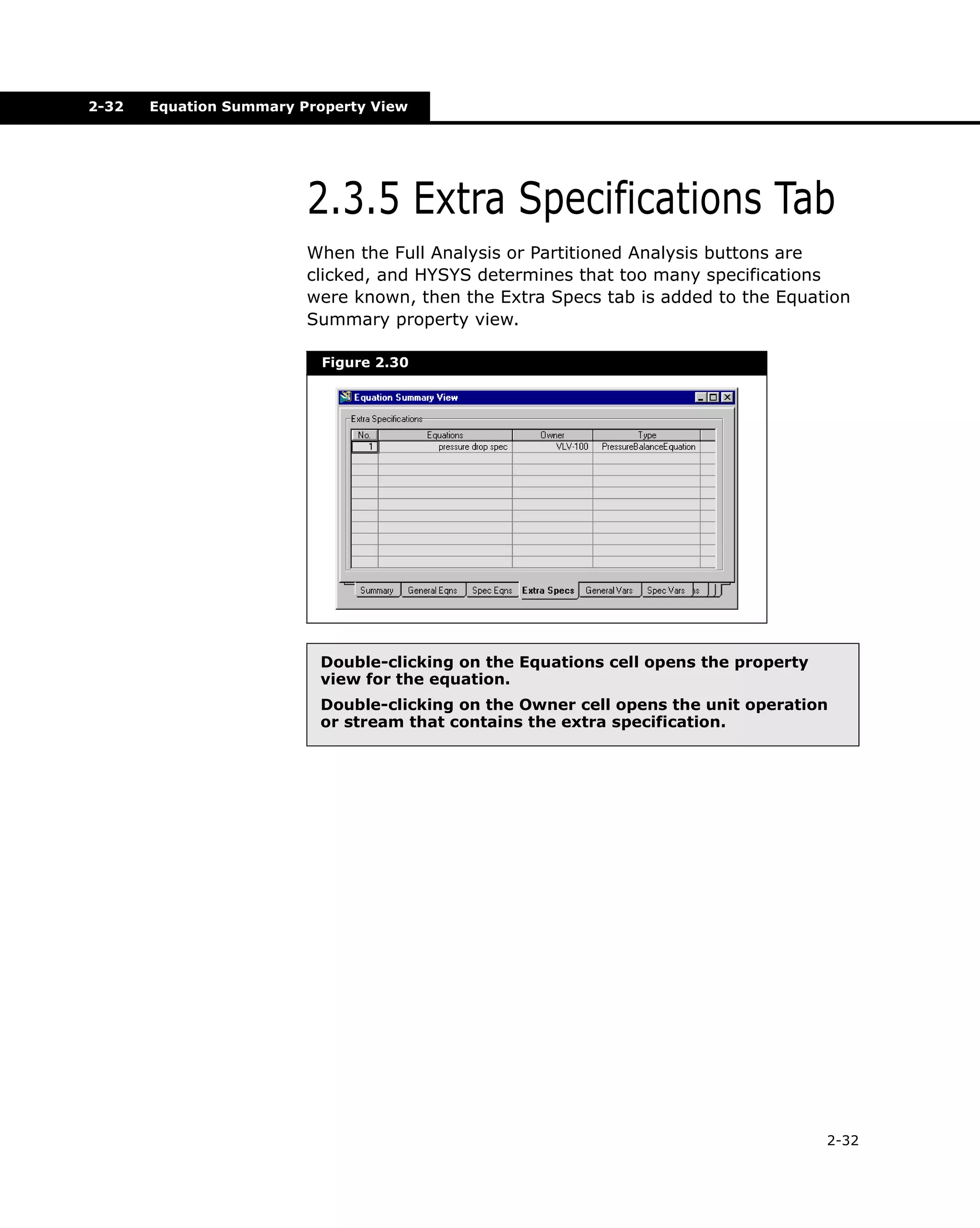
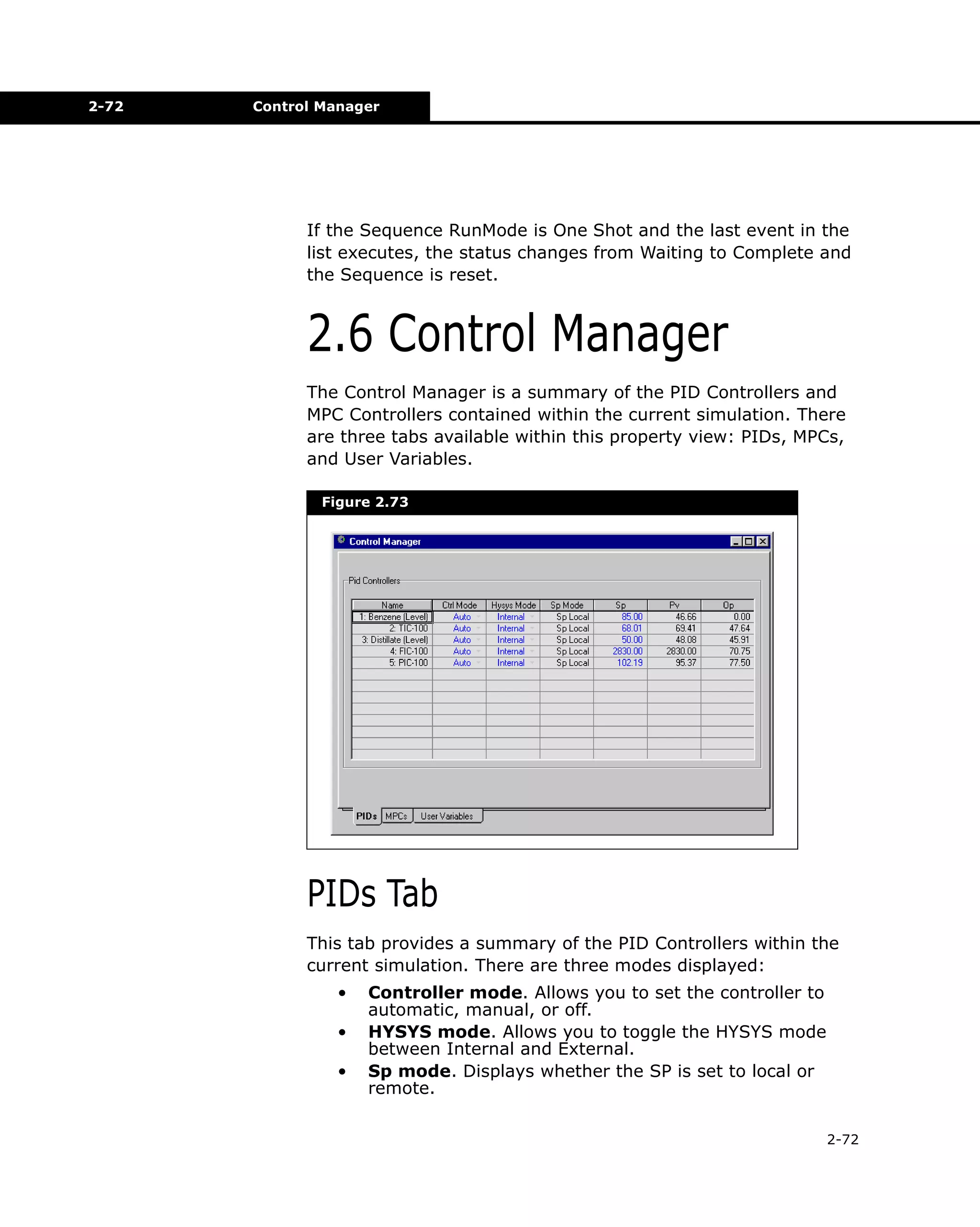
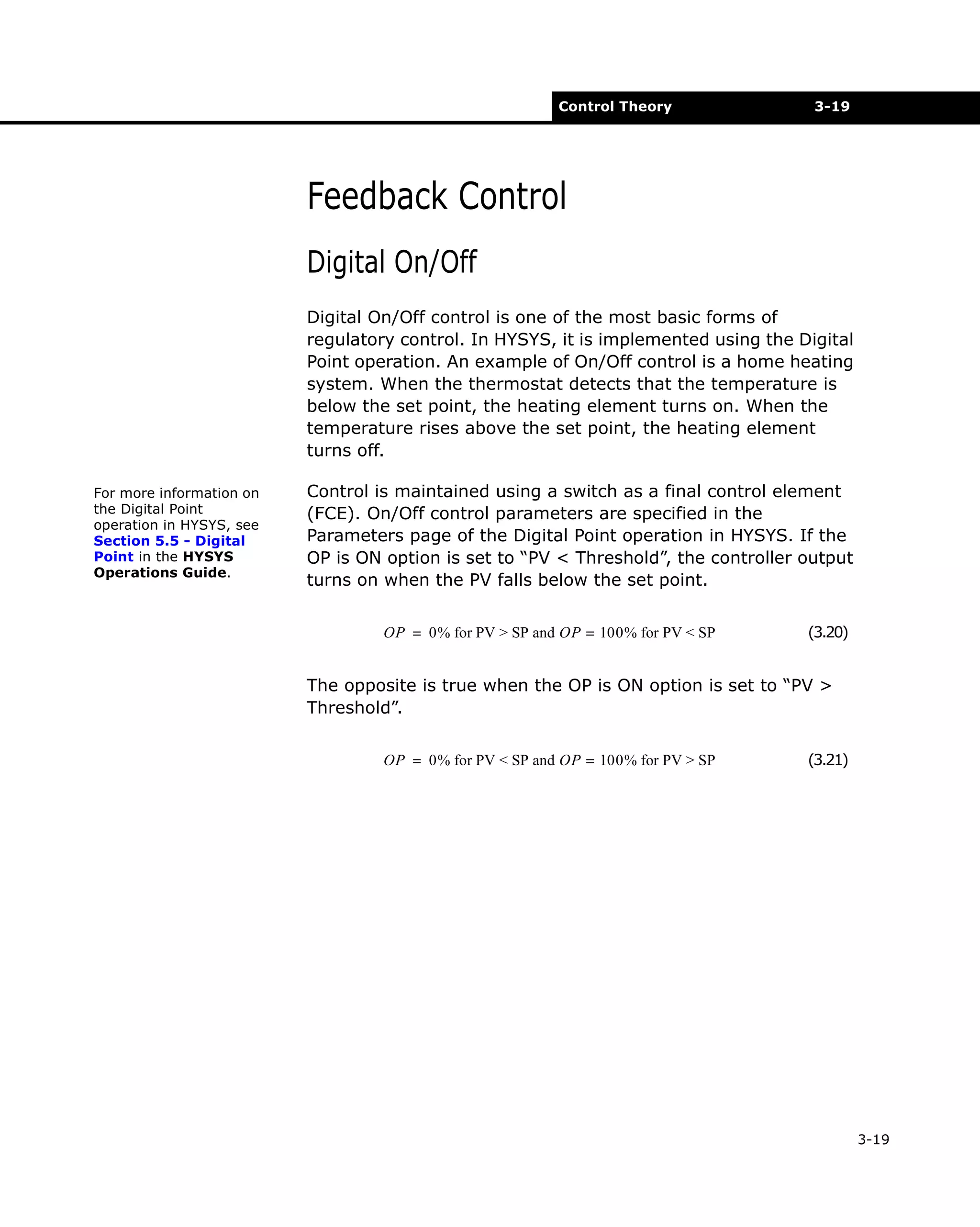
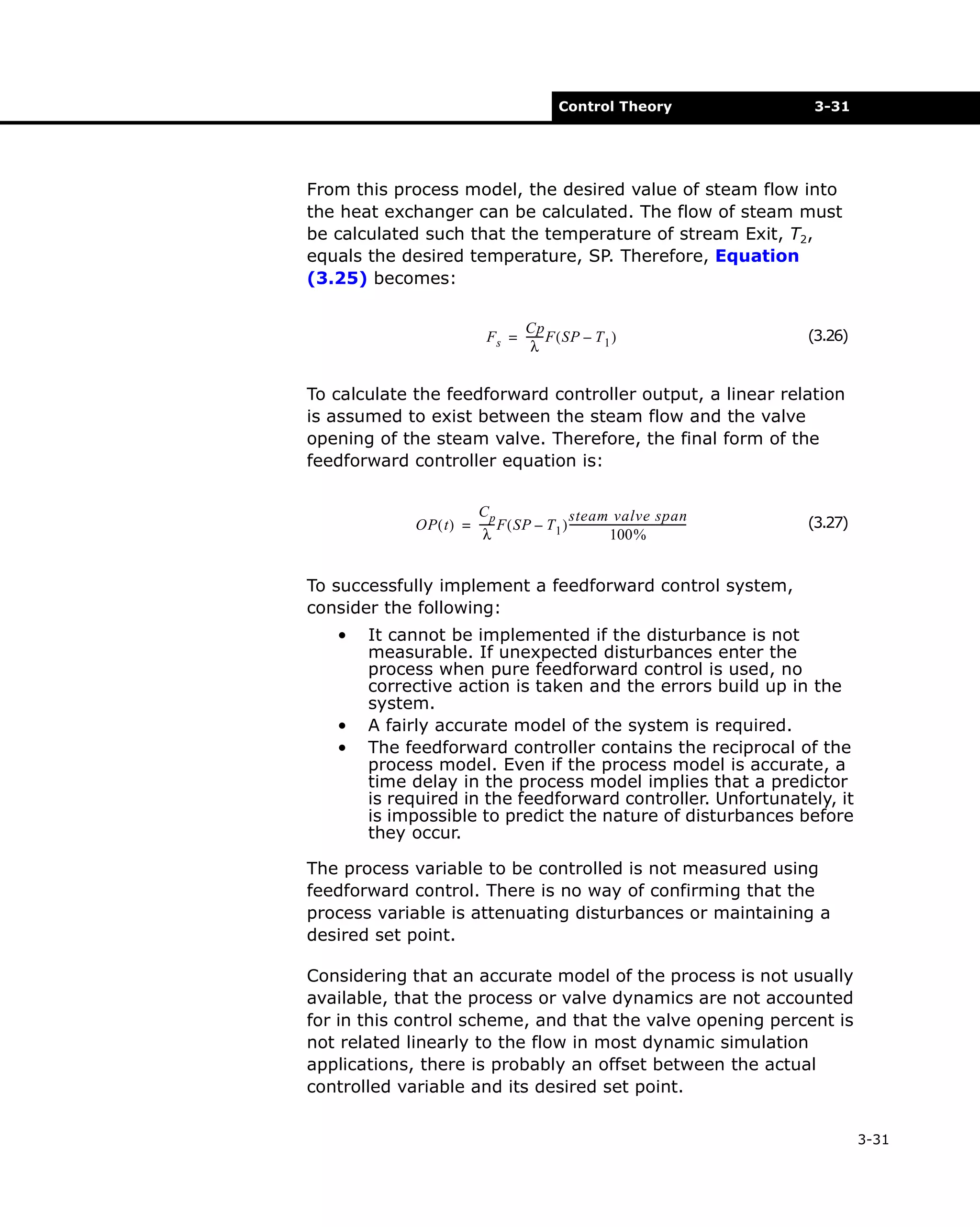
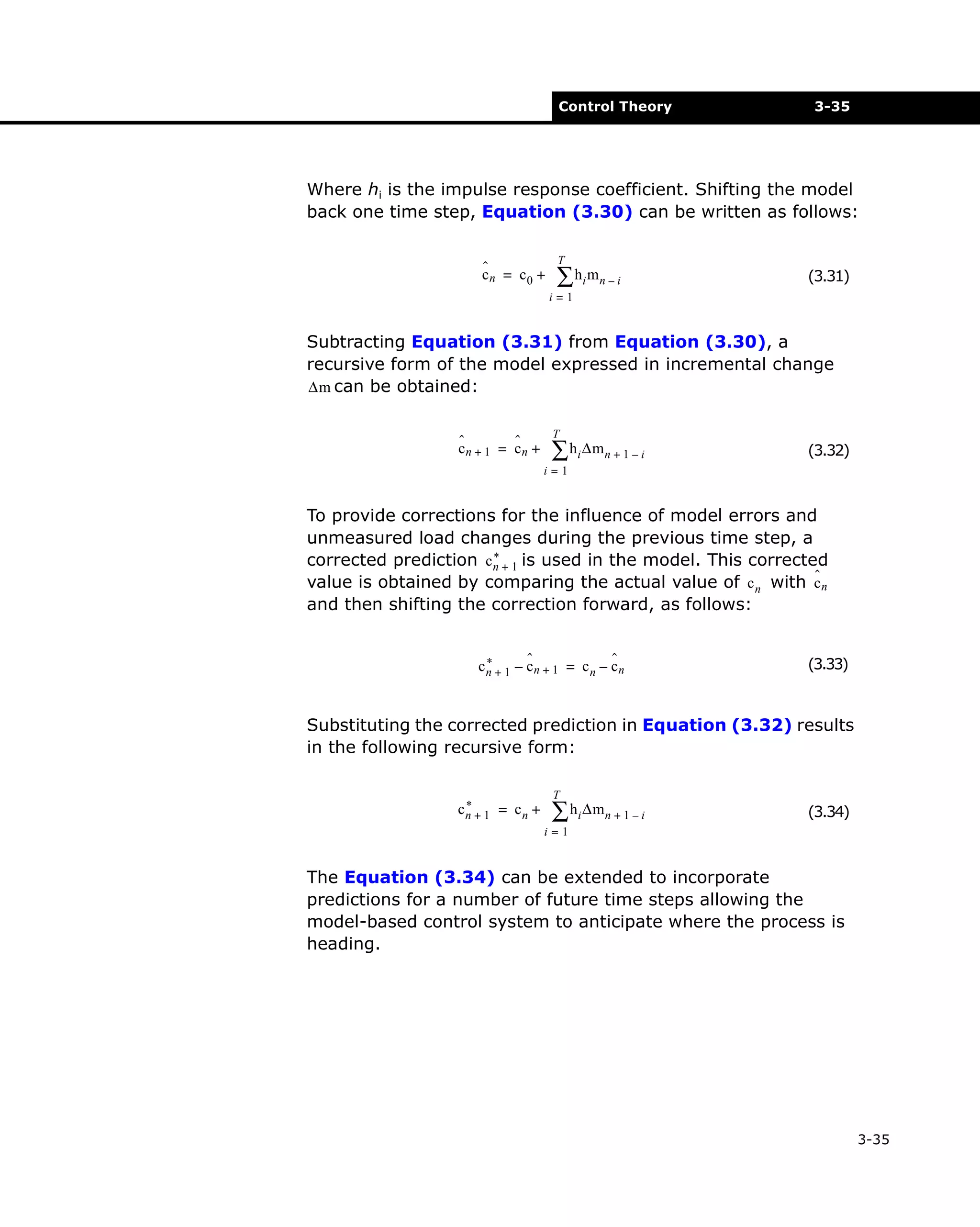
![Dynamic Theory
1-11
The general energy balance for a 2-phase system is as follows:
d [ ρ V H + ρ V h ] = F ρ h –F ρ h –F ρ H + Q + Q
l l
i i i
l l
v v
r
dt v v
(1.10)
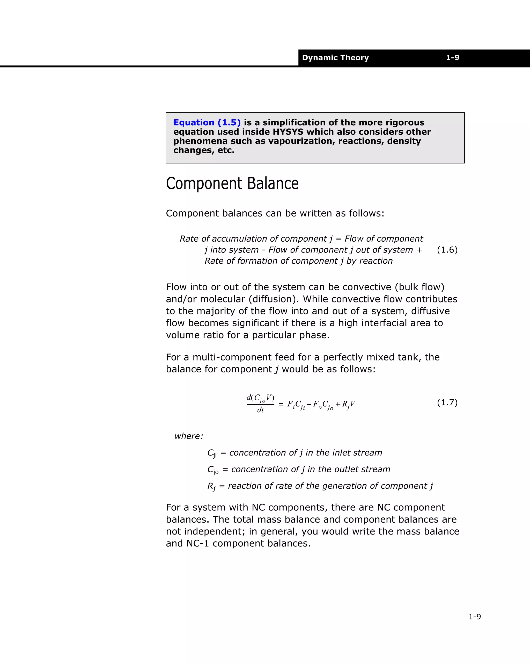
Solution Method
Implicit Euler Method
Yn+1 is analytically calculated to equal:
tn + 1
Yn + 1 = Yn +
∫
f ( Y ) dt
(1.11)
tn
where:
dY
----- = f ( Y )
dt
Ordinary differential equations are solved using the Implicit
Euler method. The Implicit Euler method is simply an
approximation of Yn+1 using rectangular integration. Graphically,
a line of slope zero and length h (the step size) is extended from
tn to tn+1 on an f(Y) vs. time plot. The area under the curve is
approximated by a rectangle of length h and height fn+1(Yn+1):
Y n + 1 = Y n + hf n + 1 ( Y n + 1 )
(1.12)
1-11](https://image.slidesharecdn.com/aspenhysysdynamicmodeling-140221173504-phpapp02/75/Aspen-hysys-dynamic-modeling-18-2048.jpg)
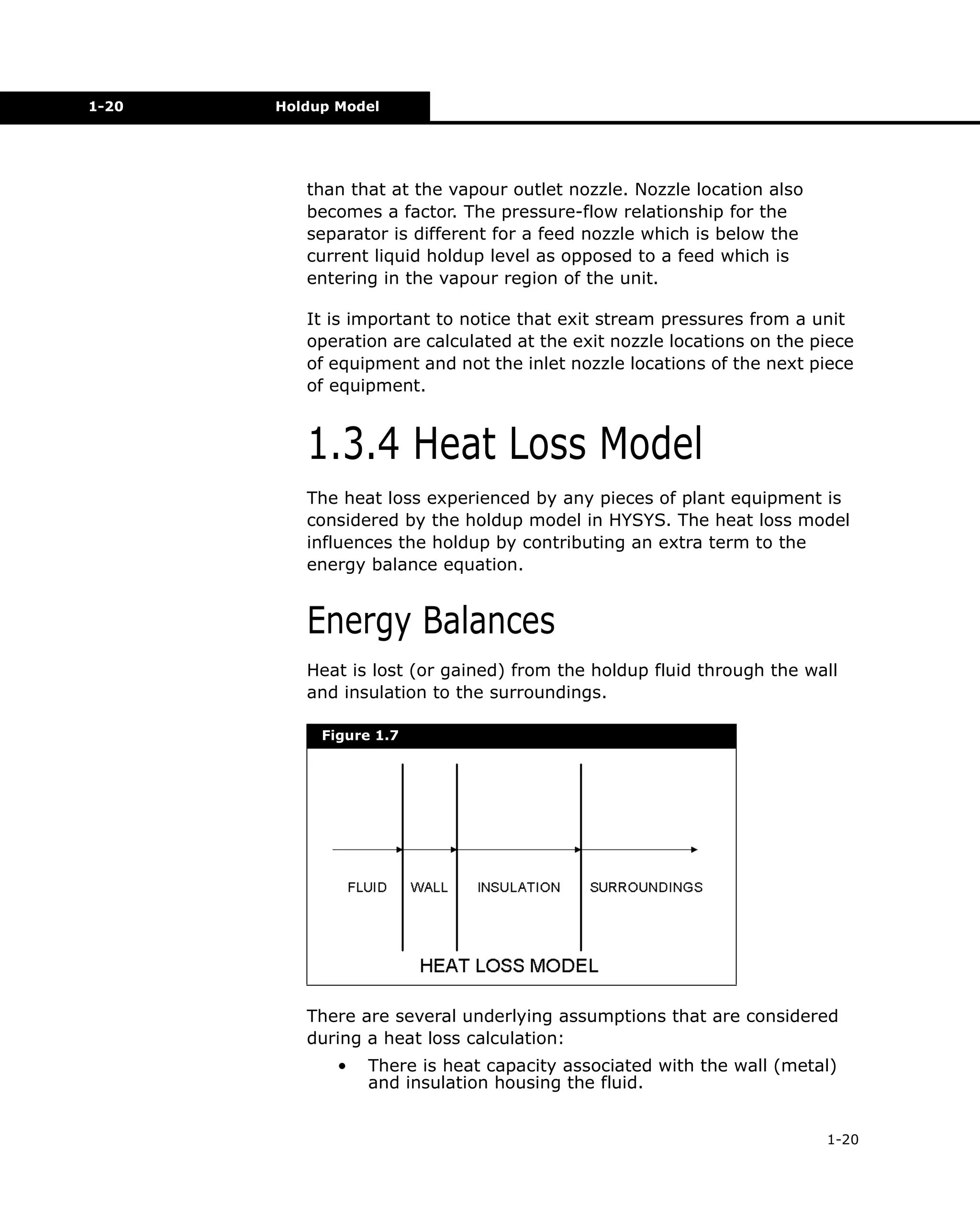
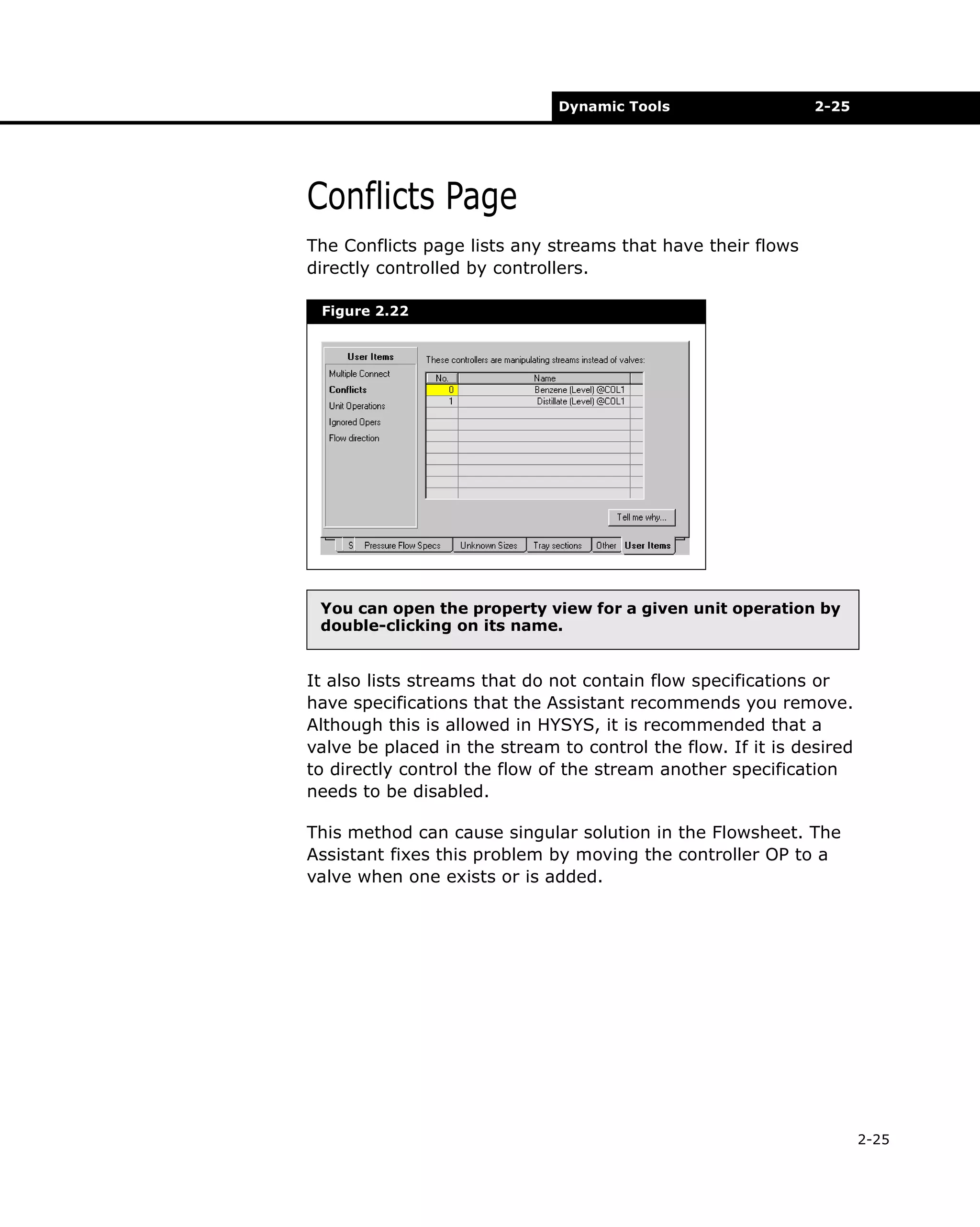
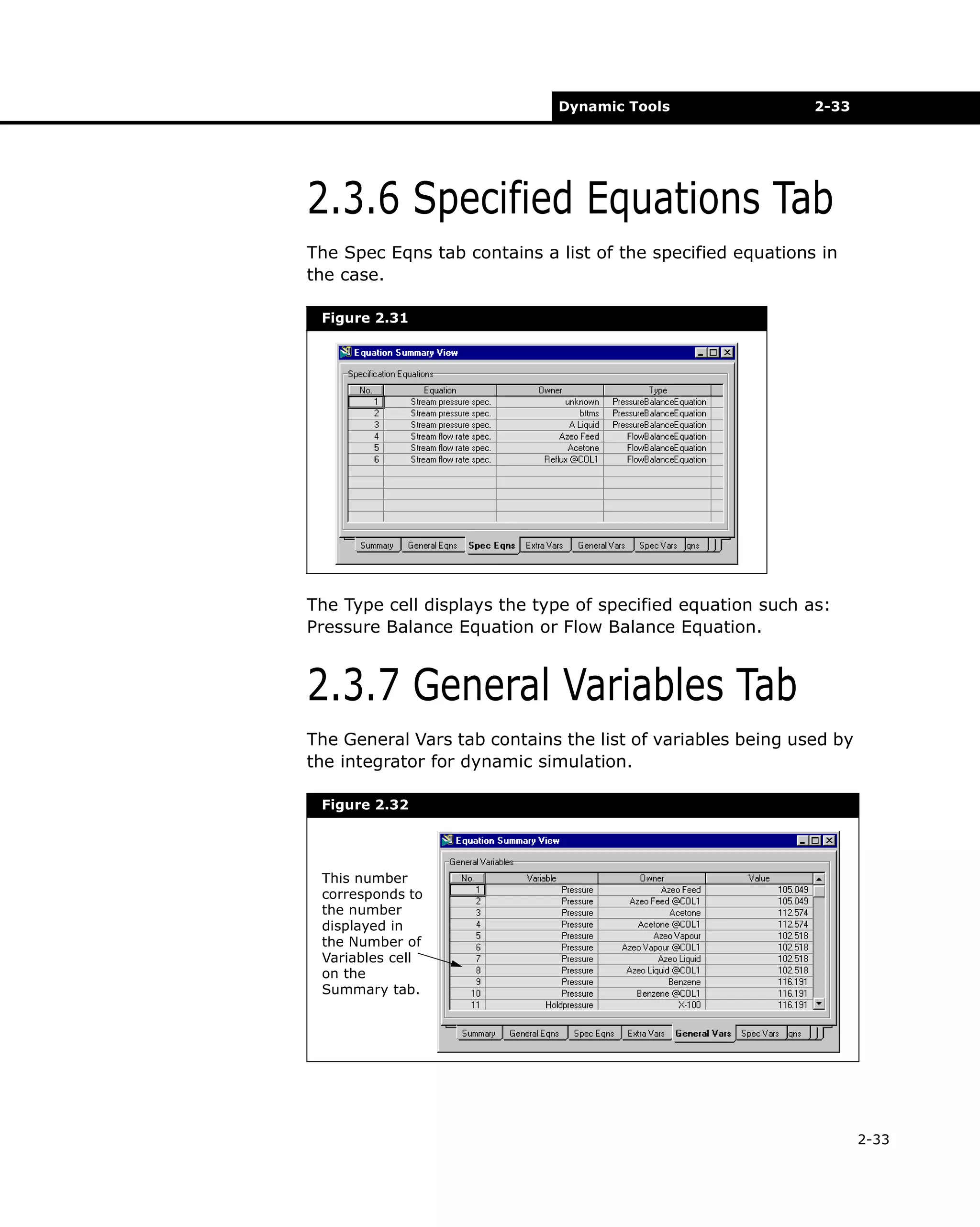
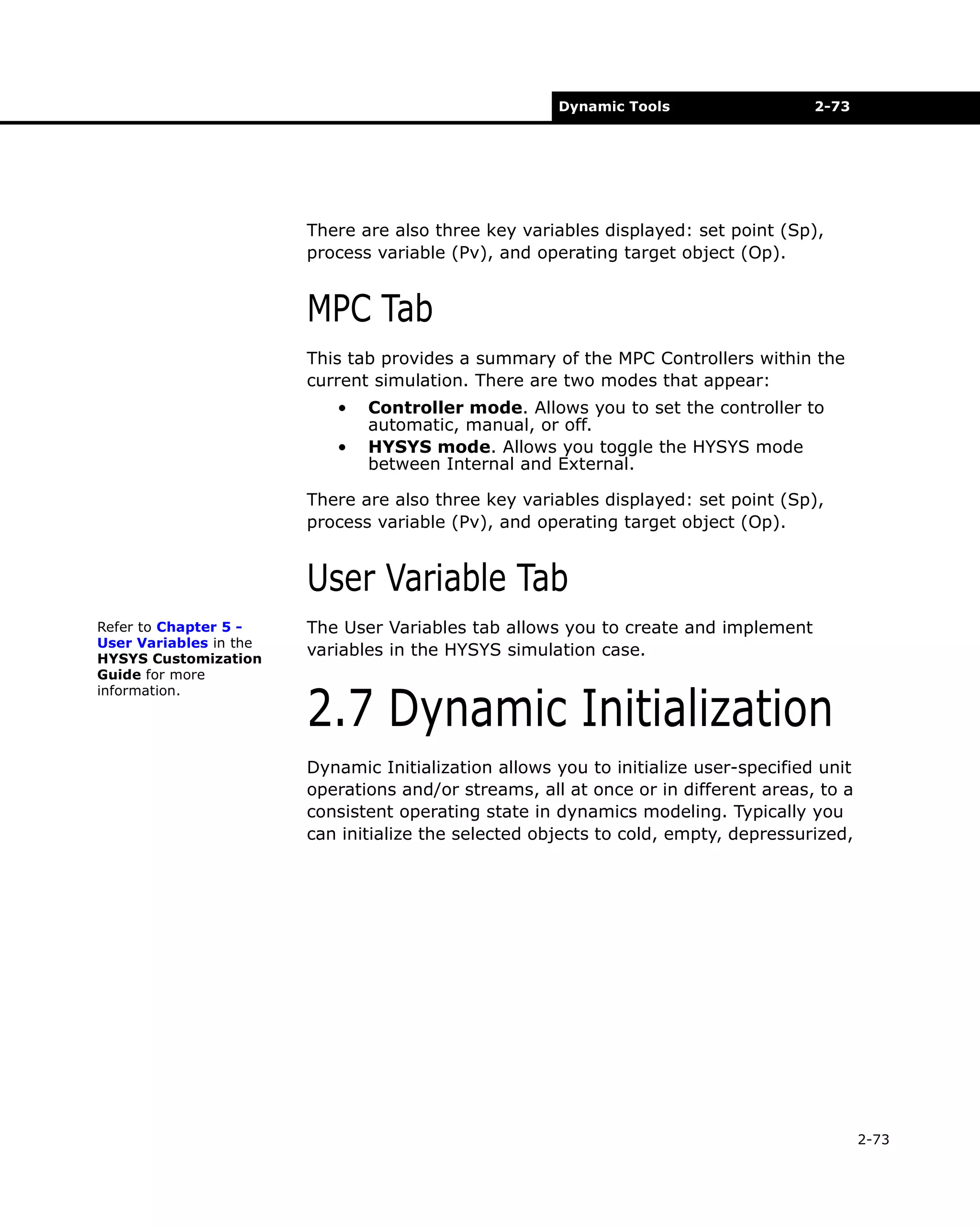
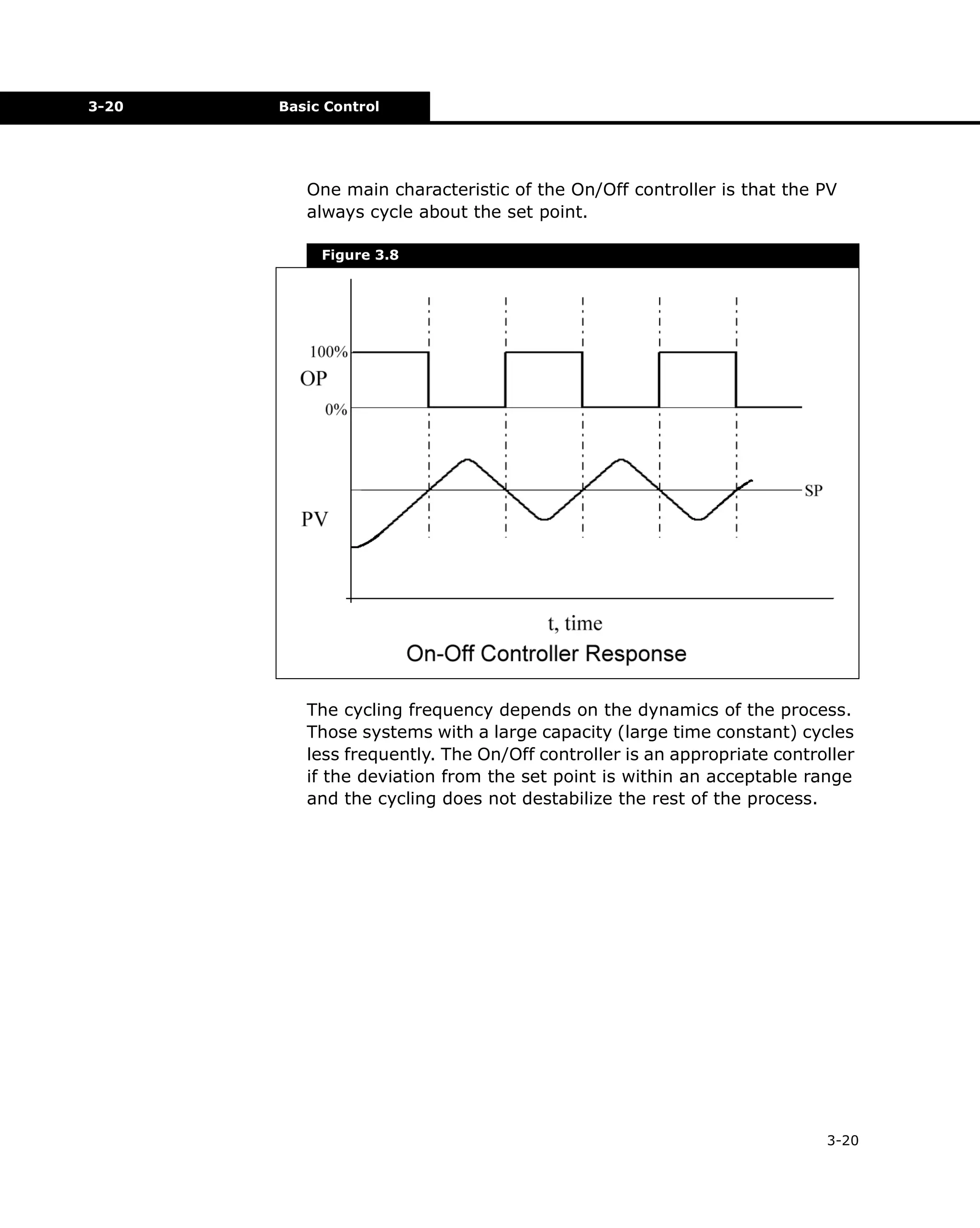
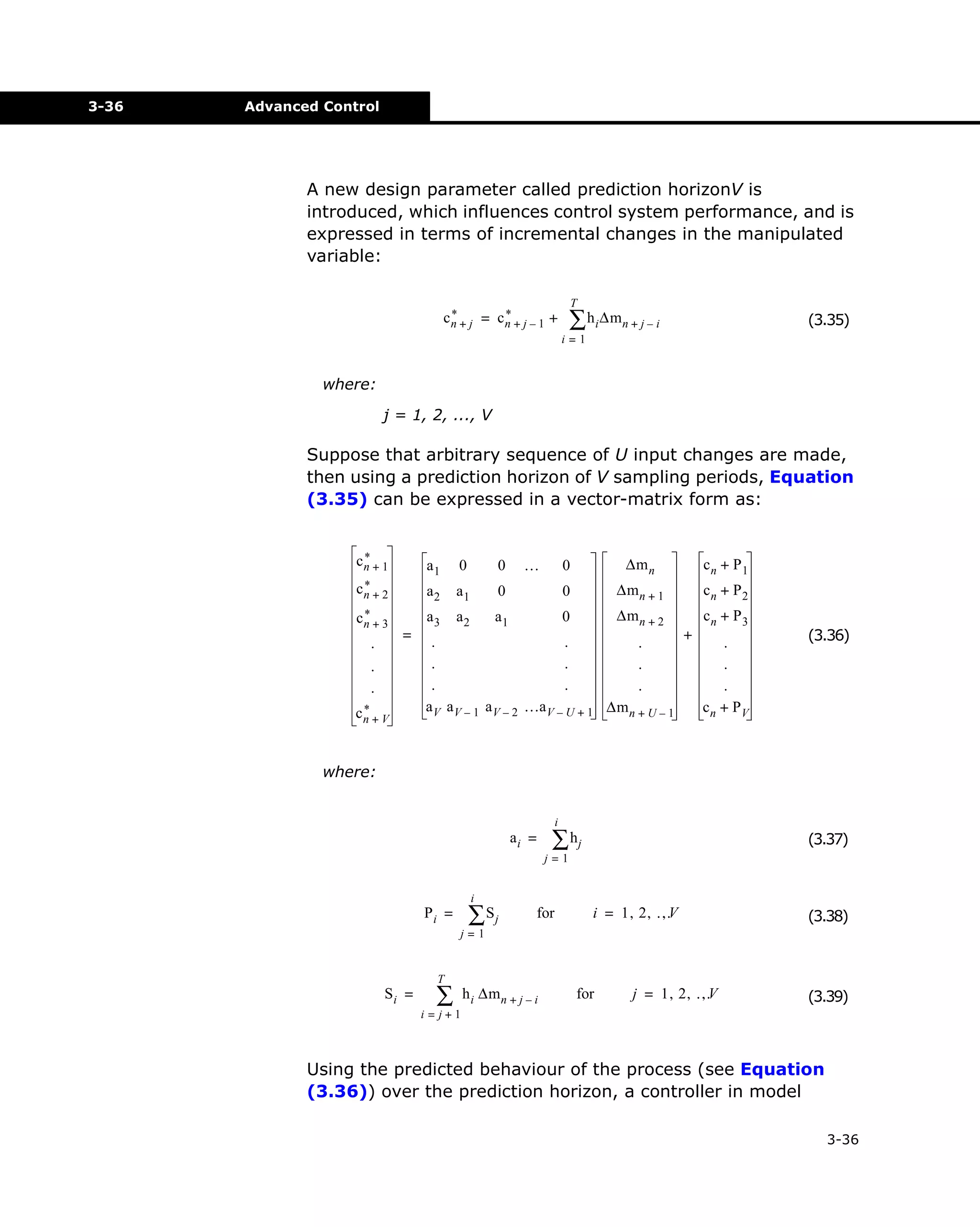
![Dynamic Theory
•
•
•
•
•
1-21
There is thermal conductivity associated with the wall
and insulation housing the fluid.
The temperature across the wall and insulation is
assumed to be constant (lumped parameter analysis).
You can now have different heat transfer coefficients on
the inside of a vessel for the vapour and the liquid. The
heat transfer coefficient between the holdup and the wall
is no longer assumed to be same for the vapour and
liquid.
The calculation uses convective heat transfer on the
inside and outside of the vessel.
The calculations assume that the temperature does not
vary along the height of the vessel, and there is a
temperature gradient through the thickness of the wall
and insulation.
A balance can be performed across the wall:
d
[ Ax wall Cp wall T wall ] = h ( fluid,
dt
wall ) A ( T fluid
k ins
– T wall ) – -------- A ( T wall – T ins )
x ins
(1.14)
The balance across the insulation is:
T ins
d
Ax ins Cp ins ---------
2
dt
k ins
= -------- A ( T wall – T ins ) + h ( ins,
x ins
surr ) A ( T ins
– T surr )
(1.15)
where:
A = the heat transfer area
x = the thickness
Cp = the heat capacity
T = the temperature
k = the thermal conductivity
h = the heat transfer coefficient
As shown, both the insulation and wall can store heat. The heat
loss term that is accounted for in the energy balance around the
holdup is h ( fluid, wall ) A ( Tfluid – T wall ) . If Tfluid is greater than Twall, the
heat is lost to the surroundings. If Tfluid is less than Twall, the heat
is gained from the surroundings.
1-21](https://image.slidesharecdn.com/aspenhysysdynamicmodeling-140221173504-phpapp02/75/Aspen-hysys-dynamic-modeling-28-2048.jpg)


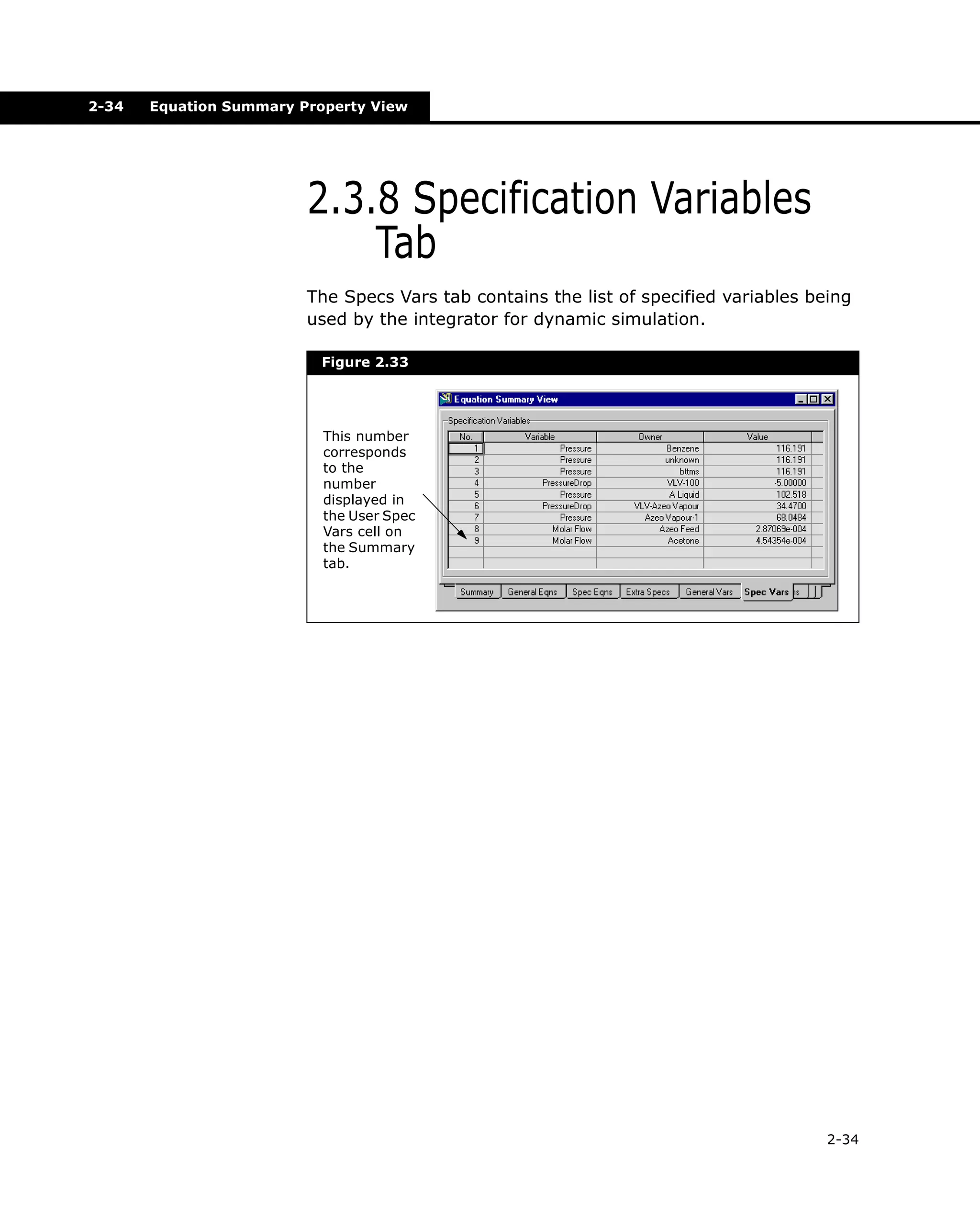
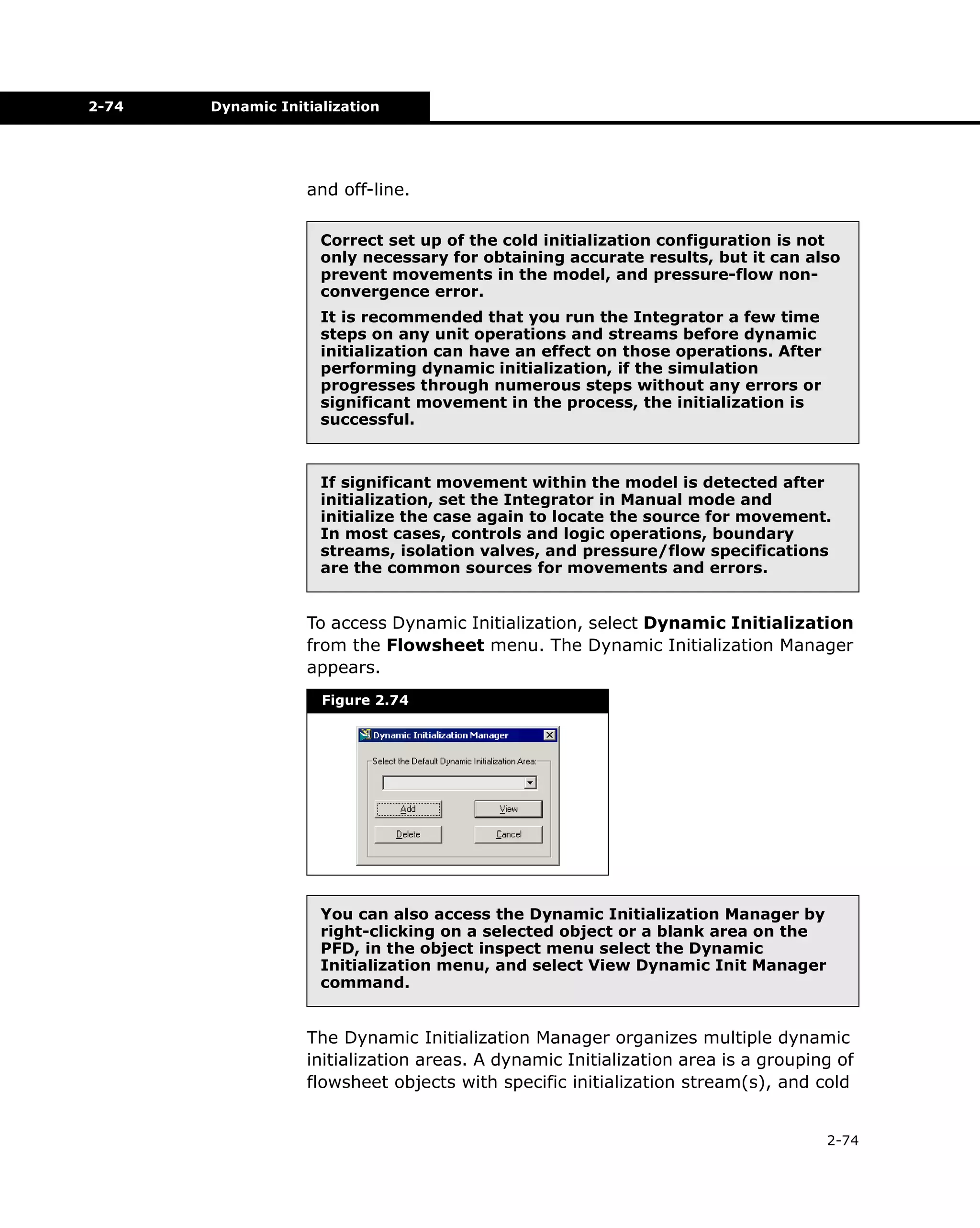

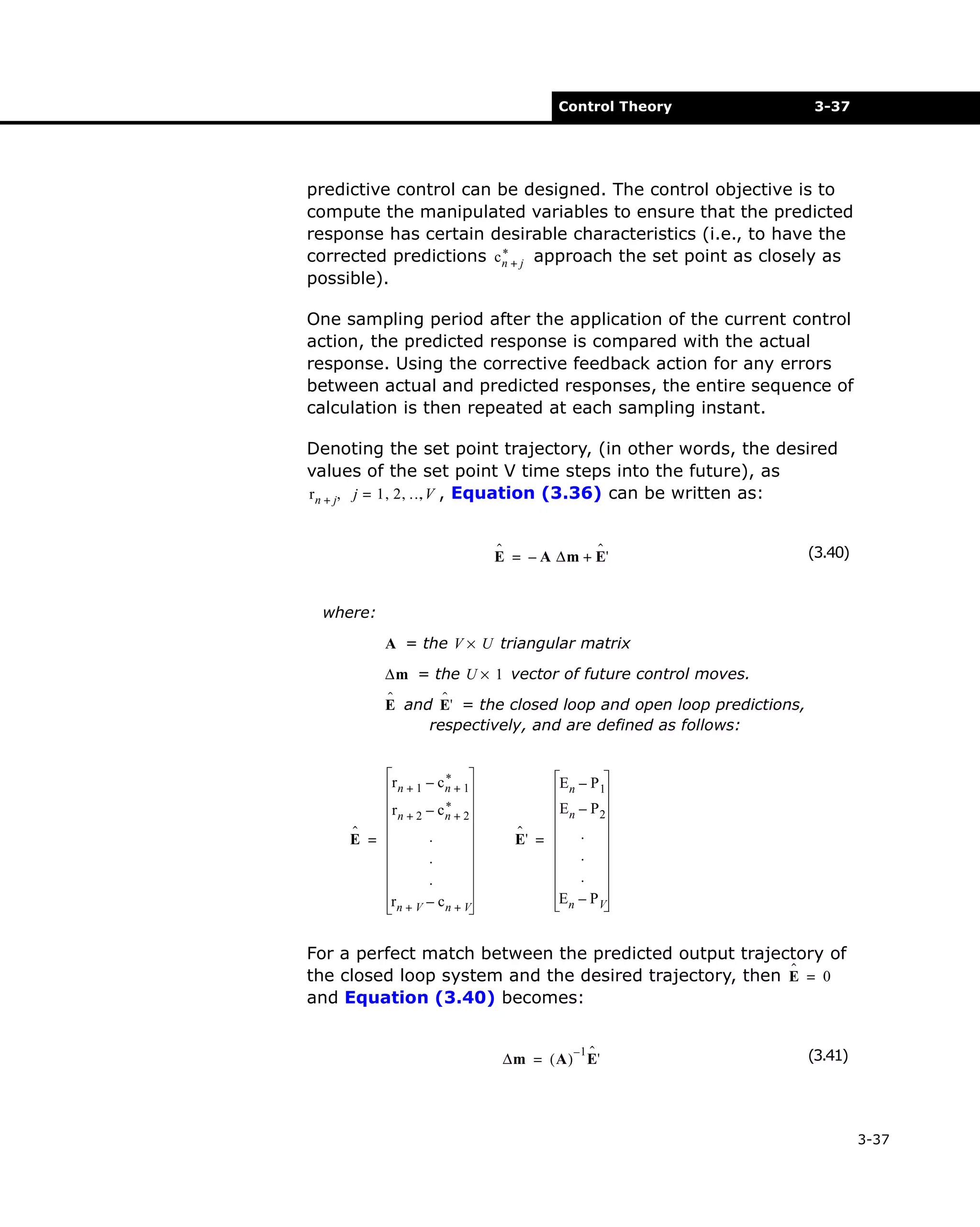
![3-38
Advanced Control
The best solution can be obtained by minimizing the
performance index:
ˆ ˆ
J [ ∆m ] = E T E
(3.42)
Here, the optimal solution for an over-determined system ( U < V )
turns out to be the least squares solution and is given by
–1
ˆ
ˆ
∆m = ( A T A ) A T E' = K c E'
(3.43)
where:
–1
( A T A ) A T = pseudo-inverse matrix
K c = matrix of feedback gains (with dimensions V × U )
One of the shortcomings of Equation (3.42) is that it can result
in excessively large changes in the manipulated variable, when
A T A is either poorly defined or singular. One way to overcome
this problem is by modifying the performance index by
penalizing movements of the manipulated variable.
ˆ
ˆ
J [ ∆m ] = E T Γ u E + ∆m T Γ y ∆m
(3.44)
where:
Γ u and Γ y are positive-definite weighting matrices for
predicted errors and control moves, respectively. These
matrices allows you to specify different penalties to be
placed on the predicted errors resulting in a better
tuned controller.
The resulting control law that minimizes J is
–1
ˆ
ˆ
∆m = ( A T Γ u A + Γ y ) A T Γ u E' = K c E'
(3.45)
The weighting matrices Γ u and Γ y contains a potentially large
number of design parameters. It is usually sufficient to select
Γ u = I and Γ y = f I ( I is the identity matrix and f is a scalar
3-38](https://image.slidesharecdn.com/aspenhysysdynamicmodeling-140221173504-phpapp02/75/Aspen-hysys-dynamic-modeling-201-2048.jpg)


![Enabling model based decision support[1]](https://cdn.slidesharecdn.com/ss_thumbnails/enablingmodel-baseddecisionsupport1-120713034639-phpapp01-thumbnail.jpg?width=640&height=640&fit=bounds)


