Downloaded 314 times
![Page 1 of 14
Process Design for Natural Gas Transmission
Jayanthi Vijay Sarathy, M.E, CEng, MIChemE, Chartered Chemical Engineer, IChemE, UK
Compressor stations form a keyl part of the
natural gas pipeline network that moves
natural gas from individual producing well
sites to end users. As natural gas moves
through a pipeline, distance, friction, and
elevation differences slow the movement of
the gas, and reduce pressure. Compressor
stations are placed strategically within the
gathering and transportation pipeline
network to help maintain the pressure and
flow of gas to market. The following is a
tutorial to perform process design of a
natural gas transmission system.
Problem Statement
80 MMscfd of Natural Gas at 36 bara & 480C is
to be transmitted from a gas plant in a desert
region to a city power station located 50 km
away. The gas composition & critical
properties are as follows,
Table 1. Natural Gas Composition & Properties
Component MW Mol% Pc,i Tc,i
- kg/kmol % psia 0R
Methane 16.04 76.23 667.8 343.0
Ethane 30.07 10.00 707.8 549.8
Propane 44.01 5.00 616.3 665.7
i-Butane 58.12 1.00 550.7 765.3
n-Butane 58.12 1.00 529.1 734.6
i-Pentane 72.15 0.30 490.4 828.7
n-Pentane 72.15 0.10 488.6 845.3
n-Hexane 86.18 0.05 436.9 913.3
C7+ 119.00 0.05 453.0 1116.0
H2O 18.02 0.25 3206.2 1164.9
CO2 44.01 3.00 1071.0 547.5
H2S 34.08 0.02 1306.0 672.3
N2 28.01 3.00 493.0 226.97
During transmission, gas pressure drops for
which a booster station is installed en-route.
The minimum pressure required at the
booster station is 10 bara & the ambient
pressure and temperature is 1.01325 bara &
300C. The design pressure & design
temperature of the pipeline-compressor
transmission system is 40 bara & 2000C.
The requirement to be met for pipeline wall
stresses is ASME B31.8. As per ASME B31.8,
the Design factor [F], Temperature De-rating
[T], Longitudinal Joint Factor [E] for the
chosen pipeline joining methods is as follows,
Table 2. Reference Mechanical Design Parameters
Design Factors [F] - Gas Pipeline Location
Class Description F
Class 1, Div 1 Deserted 0.80
Class 1, Div 2 Deserted 0.72
Class 2 Village 0.60
Class 3 City 0.50
Class 4 Densely Populated 0.40
Temperature De-rating [T] for Gas Pipelines
T [0F] T [0C] T
250 120 1.00
300 150 0.97
350 175 0.93
400 200 0.91
450 230 0.87
Abbreviation Joining Method E
SMLS Seamless 1.0
ERW Electric Resistance Weld 1.0
EFW Electric Flash Weld 1.0
SAW Submerged Arc Weld 1.0
BW Furnace Butt Weld 0.6
EFAW Electric Fusion Arc Weld 0.8](https://image.slidesharecdn.com/naturalgastransmissiontutorial-191103080412/85/Process-Design-for-Natural-Gas-Transmission-1-320.jpg)
![Page 1 of 14
Process Design for Natural Gas Transmission
Jayanthi Vijay Sarathy, M.E, CEng, MIChemE, Chartered Chemical Engineer, IChemE, UK
Compressor stations form a keyl part of the
natural gas pipeline network that moves
natural gas from individual producing well
sites to end users. As natural gas moves
through a pipeline, distance, friction, and
elevation differences slow the movement of
the gas, and reduce pressure. Compressor
stations are placed strategically within the
gathering and transportation pipeline
network to help maintain the pressure and
flow of gas to market. The following is a
tutorial to perform process design of a
natural gas transmission system.
Problem Statement
80 MMscfd of Natural Gas at 36 bara & 480C is
to be transmitted from a gas plant in a desert
region to a city power station located 50 km
away. The gas composition & critical
properties are as follows,
Table 1. Natural Gas Composition & Properties
Component MW Mol% Pc,i Tc,i
- kg/kmol % psia 0R
Methane 16.04 76.23 667.8 343.0
Ethane 30.07 10.00 707.8 549.8
Propane 44.01 5.00 616.3 665.7
i-Butane 58.12 1.00 550.7 765.3
n-Butane 58.12 1.00 529.1 734.6
i-Pentane 72.15 0.30 490.4 828.7
n-Pentane 72.15 0.10 488.6 845.3
n-Hexane 86.18 0.05 436.9 913.3
C7+ 119.00 0.05 453.0 1116.0
H2O 18.02 0.25 3206.2 1164.9
CO2 44.01 3.00 1071.0 547.5
H2S 34.08 0.02 1306.0 672.3
N2 28.01 3.00 493.0 226.97
During transmission, gas pressure drops for
which a booster station is installed en-route.
The minimum pressure required at the
booster station is 10 bara & the ambient
pressure and temperature is 1.01325 bara &
300C. The design pressure & design
temperature of the pipeline-compressor
transmission system is 40 bara & 2000C.
The requirement to be met for pipeline wall
stresses is ASME B31.8. As per ASME B31.8,
the Design factor [F], Temperature De-rating
[T], Longitudinal Joint Factor [E] for the
chosen pipeline joining methods is as follows,
Table 2. Reference Mechanical Design Parameters
Design Factors [F] - Gas Pipeline Location
Class Description F
Class 1, Div 1 Deserted 0.80
Class 1, Div 2 Deserted 0.72
Class 2 Village 0.60
Class 3 City 0.50
Class 4 Densely Populated 0.40
Temperature De-rating [T] for Gas Pipelines
T [0F] T [0C] T
250 120 1.00
300 150 0.97
350 175 0.93
400 200 0.91
450 230 0.87
Abbreviation Joining Method E
SMLS Seamless 1.0
ERW Electric Resistance Weld 1.0
EFW Electric Flash Weld 1.0
SAW Submerged Arc Weld 1.0
BW Furnace Butt Weld 0.6
EFAW Electric Fusion Arc Weld 0.8](https://image.slidesharecdn.com/naturalgastransmissiontutorial-191103080412/75/Process-Design-for-Natural-Gas-Transmission-1-2048.jpg)
![Page 2 of 14
The pipeline specification requirement is API
5L plain end line pipe specifications ranging
from 6” ND to 80” ND. The product pipeline
specification (PSL) with its respective
Specified Minimum Yield Strength (SYMS) to
be used as per API 5L are PSL 1 and PSL 2.
The pipeline grades are as follows,
Table 3. Product Specification Level (PSL)
Grade
SMYS
Grade
SMYS
MPa MPa
PSL 1 Gr A25 172 PSL 2 Gr B 241
PSL 1 Gr A 207 PSL 2 X42 290
PSL 1 Gr B 241 PSL 2 X46 317
PSL 1 X42 290 PSL 2 X52 359
PSL 1 X46 317 PSL 2 X56 386
PSL 1 X52 359 PSL 2 X60 414
PSL 1 X56 386 PSL 2 X65 448
PSL 1 X60 414 PSL 2 X70 483
PSL 1 X65 448 PSL 2 X80 552
PSL 1 X70 483 - -
In the current tutorial, the API 5L pipeline
grades chosen for both desert location [Class
1, F = 0.72] & city location [Class 3, F = 0.50]
is PSL 1 X65 [SMYS = 448 Mpa]. The pipeline
joining method chosen is Electric Resistance
Weld [ERW] with a longitudinal joining factor
[E] of 1.0. The temperature de-rating factor
[T] of the pipelines before & after the booster
station for a design temperature of 2000C as
per Table 2 is 0.91. The design capacity of the
pipeline is taken as 100 MMscfd.
For the tutorial, the pipelines before & after
the booster station is laid below ground that
has a constant soil temperature of 300C & soil
overall heat transfer coefficient [U] of 35
W/m2.K. The pipeline corrosion allowance
before & after the booster station is taken as
3 mm considering a corrosion rate of 5
mils/year [1 mil = 1/1000th of an inch] over a
25 year operating period.
The pipeline would include fittings and
elevational differences which offer a pressure
drop & hence can be expressed as an
equivalent length. For this tutorial, the fittings
& elevation losses are taken as 2% of the total
pipeline length. The booster compressor
station is placed at a distance of 20km from
the gas plant located in the desert area & the
downstream pipeline travels another 30 km
to reach the power station in the city. This is
shown as follows,
Table 4. Pipeline Lengths
Pipeline Length Eq. Length
Total Eq.
Length
- [m] [%] [m] [m]
Upstream 20,000 2 400 20,400
Downstream 30,000 2 600 30,600
It is assumed that the condensation in the
pipeline is minimal and hence the pipeline
efficiency [Ep] is taken as 0.92. To evaluate
the maximum hydrostatic test pressure, the
difference in elevation of the pipeline
between the pipeline high point elevation and
elevation at test point for upstream and down
stream pipelines is taken as 100m and 70m &
100m and 90m respectively.
The pipeline booster station consists of a
centrifugal compressor operating with
polytropic efficiency [p] of 80% at 80
MMscfd. The minimum pressure required at
the compressor inlet is 12 bara & a minimum
pressure of 16 bara at the city power station.
Design Methodology
To perform a process design of the pipeline &
booster compressor station, the design
methodology consists of 3 parts – Process
design of upstream pipeline from the gas
plant from the desert, process design of the
gas compressor at the booster station and
downstream pipeline to the city power
station. The process design steps for the
upstream/downstream pipelines are,](https://image.slidesharecdn.com/naturalgastransmissiontutorial-191103080412/85/Process-Design-for-Natural-Gas-Transmission-2-320.jpg)
![Page 3 of 14
1. Estimation of Pipeline wall thickness based
on design pressure [DP], design
temperature [DT], design flowrate [Qd],
location class, design factor [F], pipeline
specification [API 5L], specified minimum
yield strength [SMYS], derating factor [T].
2. Estimation of Mixture Pseudocritical
Properties – Pseudo critical Pressure [Tc],
Pseudo critical Temperature [Tc], Reduced
Pressure [Ppr], Reduced Temperature [Tpr],
Reduced Density [r], Deviation Parameter
[], Modified Reduced Pressure [P’pc],
Modified Reduced Temperature [T’pc],
Specific Heat Capacity [Cp], Gas
Compressibility Factor [Z].
3. Estimation of gas mixture density [],
mixture molecular weight [MW], mass flow
[m] and actual volumetric flow rate [Q].
4. Estimation of Upstream/Downstream
Pipeline Fluid Velocity [V], Pipeline Exit
Temperature [Pe] based on soil/ambient
temperature, overall heat transfer co-
efficient [U], Pipeline Pressure drop [P],
Pipeline Exit Pressure & Pressure drop per
km [P/L].
5. Estimation of Maximum Allowable
Operating Pressure [MAOP], Test Pressure
at 110% of SMYS, Maximum Hydrostatic
Test Pressure & Leak Test Pressure.
For the Booster Compressor Station, the
design steps are,
1. Estimation of Mixture Critical Properties –
Pseudocritical Pressure [Tc], Pseudocritical
Temperature [Tc], Reduced Pressure [Ppr],
Reduced Temperature [Tpr], Reduced
Density [r], Deviation Parameter [],
Modified Reduced Pressure [P’pc], Modified
Reduced Temperature [T’pc], Specific Heat
Capacity [Cp], Gas Compressibility [Z].
2. Estimation of Adiabatic Exponent [k],
compressor inlet gas mixture density [],
average polytropic exponent [n] based on
polytropic efficiency [p], adiabatic
efficiency [a], molar density [[m], molar
volume [Vm], mass flow [m], Molar flow
[M], Polytropic Head [Hp] & Absorbed
Power [P].
3. Check if compressor energy balance
condition, P1V1
n-P2V2
n = 0 is satisfied.
4. Repeat above steps for compressor
discharge side for process parameters.
Property Estimation Methodology
To assess the properties of natural gas,
calculations can be begun by estimating the
properties using Kay’s Mixing Rule as follows,
Mixture molecular weight [MW], kg/kmol
𝑀𝑊 = ∑ 𝑦𝑖 𝑀𝑊𝑖 (1)
Mixture Pseudo Critical Pressure [Pc], psia
𝑃𝑐 = ∑ 𝑦𝑖 𝑃𝑐,𝑖 (2)
Mixture Pseudo Critical Temperature [Tc], 0R
𝑇𝑐 = ∑ 𝑦𝑖 𝑇𝑐,𝑖 (3)
Gas Specific Gravity [g], [-]
𝛾𝑔 =
𝑀𝑊𝑔
𝑀𝑊 𝑎𝑖𝑟
; MWair = 28.96 kg/kmol (4)
From the above, Kay’s Mixing Rule does not
give accurate pseudocritical properties for
higher molecular weight mixtures
(particularly C7+ mixtures) of hydrocarbon
gases when estimating gas compressibility
factors [Z] and deviations can be as high as
15%. Therefore, to account for these
differences, Sutton’s correlations based on
gas specific gravity can be utilized as follows,
𝑃𝑝𝑐 = 756.8 − 131.07𝛾𝑔 − 3.6𝛾𝑔
2
(5)
𝑇𝑝𝑐 = 169.2 − 349.5𝛾𝑔 − 74.0𝛾𝑔
2
(6)
The above equations are valid for the gas
specific gravities range of 0.57 < g < 1.68.
Using the Sutton correlations, the reduced
properties are calculated as,
𝑃𝑟 =
𝑃
𝑃 𝑝𝑐
(7)
𝑇𝑟 =
𝑇
𝑇𝑝𝑐
(8)](https://image.slidesharecdn.com/naturalgastransmissiontutorial-191103080412/85/Process-Design-for-Natural-Gas-Transmission-3-320.jpg)
![Page 4 of 14
However the pseudocritical properties are
not the actual mixture critical temperature
and pressure but represent the values that
must be used for the purpose of comparing
corresponding states of different gases on
the compressibility factor, Z-chart/Gas
Deviation Factor, as shown below in the
Standing & Katz, 1959 chart for natural gases.
Figure 1. Natural Gas deviation factor chart
(Standing & Katz, 1959)
Due to the graphical method of Standing &
Katz chart, the Z factor can be estimated using
Dranchuk and Abou-Kassem Equation of State
[DAK-EoS] which is based on the data of
Standing & Katz, 1959 and is expressed as,
𝑍 = 1 + [𝐴1 +
𝐴2
𝑇𝑟
+
𝐴3
𝑇𝑟
3 +
𝐴4
𝑇𝑟
4 +
𝐴5
𝑇𝑟
5] 𝜌 𝑟 +
[𝐴6 +
𝐴7
𝑇𝑟
+
𝐴8
𝑇𝑟
2] 𝜌 𝑟
2
− 𝐴9 [
𝐴7
𝑇𝑟
+
𝐴8
𝑇𝑟
2] 𝜌 𝑟
5
+
+𝐴10(1 + 𝐴11 𝜌 𝑟
2) (
𝜌 𝑟
2
𝑇𝑟
3) 𝑒−𝐴11 𝜌 𝑟
2
(9)
Where,
𝜌 𝑟 =
0.27𝑃𝑟
𝑍𝑇𝑟
(10)
r = Pseudo-Reduced Density [-]
Tr = Pseudo-Reduced Temperature [-]
And the constants A1 to A11, are as follows,
Table 5. DAK EoS A1 to A11 Constants
A1 0.3265 A7 –0.7361
A2 –1.0700 A8 0.1844
A3 –0.5339 A9 0.1056
A4 0.01569 A10 0.6134
A5 –0.05165 A11 0.7210
A6 0.5475
DAK-EoS has an average absolute error of
0.486% in its equation, with a standard
deviation of 0.00747 over ranges of pseudo-
reduced pressure and temperature of 0.2 <
Ppr < 30; 1.0 < Tpr < 3.0 and for Ppr < 1.0 with
0.7 < Tpr < 1.0. However DAK-EoS gives
unacceptable results near the critical
temperature for Tpr = 1.0 and Ppr >1.0, and
DAK EoS is not recommended in this range.
DAK EoS for NG Mixtures with Acid Gases
Natural Gas is expected to contain acid gas
fractions, such as CO2 and H2S, & applying the
Standing & Katz Z-factor chart & Sutton’s
pseudocritical properties calculation methods
would yield inaccuracies, since they are only
valid for hydrocarbon mixtures. To account
for these inaccuracies, the Wichert & Aziz
correlations can be applied to mixtures
containing CO2 < 54.4 mol% & H2S < 73.8
mol% by estimating a deviation parameter
[], which is used to modify the pseudocritical
pressure & temperatures. The deviation
parameter [] whose units are in 0R, is,
𝜀 = 120[ 𝐴0.9
− 𝐴1.6] + 15[ 𝐵0.5
− 𝐵4] (11)
Where,
A = YCO2 + YH2S in Gas mix [Y = mole fraction]
B = YH2S in Gas mixture [Y = mole fraction]
Applying [], the modified pseudocritical
pressure & temperature is,
𝑇𝑝𝑐
′
= 𝑇𝑝𝑐 − 𝜀 (12)
𝑃𝑝𝑐
′
=
𝑃 𝑝𝑐 𝑇𝑝𝑐
′
𝑇𝑝𝑐−𝐵[1−𝐵]𝜀
(13)
Where, T’pc & P’pc are valid only in 0R and psia.](https://image.slidesharecdn.com/naturalgastransmissiontutorial-191103080412/85/Process-Design-for-Natural-Gas-Transmission-4-320.jpg)
![Page 5 of 14
Based on the calculated modified
pseudocritical pressure [P’pc] and
temperature [T’pc], the pseudo-reduced
pressure [Pr] & temperature [Tr] is,
𝑃𝑝𝑟 =
𝑃 [𝑝𝑠𝑖𝑎]
𝑃𝑝𝑐
′ [𝑝𝑠𝑖𝑎]
(14)
𝑇𝑝𝑟 =
𝑇 [° 𝑅]
𝑇𝑝𝑐
′ [° 𝑅]
(15)
𝜌 𝑝𝑟 =
0.27𝑃𝑝𝑟
𝑍𝑇𝑝𝑟
(16)
Using the calculated values of Ppr Tpr & pr,
compressibility factor, Z is determined by
using DAK EoS. Owing to the value of ‘Z’ being
an implicit parameter in calculating pr as
well as in DAK-EoS, an iterative approach,
whereby Z value is guessed & iteratively
solved to satisfy both modified pseudo-
reduced density [pr] & DAK EoS. Upon
calculating the value of Zin at the pipeline
inlet, the actual volumetric flow rate [Qin], Gas
density [in], gas mass flow [m] is calculated
as follows,
Actual Volumetric Flow Rate, Am3/h
𝑄1 =
𝑃 𝑠𝑡𝑑 𝑄 𝑠𝑡𝑑 𝑍1 𝑇1
𝑍 𝑠𝑡𝑑 𝑇 𝑠𝑡𝑑 𝑃1
(17)
The value of Zstd is taken to be close to 1.0.
Gas Density, kg/m3
𝜌1 =
𝑃1 𝑀𝑊
𝑍1 𝑅𝑇1
(18)
Gas Mass Flow, kg/h
𝑚 𝑔 = 𝑄1 × 𝜌1 (19)
Pipeline Process & Mechanical Design
To perform Gas Pipeline design, dimensions
are chosen based on the following factors,
Location of the Gas Pipelines
1. Class 1 location - A Class 1 location is any
1-mile pipeline section that has 10 or
fewer buildings intended for human
occupancy including areas such as,
wastelands, deserts, rugged mountains,
grazing land, farmland, sparse populations.
2. Class 1, division 1 Location – A Class 1
location where the design factor, F, of the
pipeline is greater than 0.72 but equal to,
or less than 0.80 and which has been
hydrostatically tested to 1.25 times the
maximum operating pressure.
3. Class 1, division 2 Location - This is a
Class 1 location where the design factor, F,
of the pipeline is equal to or less than 0.72,
and which has been tested to 1.1 times the
maximum operating pressure.
4. Class 2 Location - This is any 1-mile
section of pipeline that has more than 10
but fewer than 46 buildings intended for
human occupancy including fringe areas
around cities and towns, industrial areas,
and ranch or country estates.
5. Class 3 Location - This is any 1-mile
section of pipeline that has 46 or more
buildings intended for human occupancy
except when a Class 4 Location prevails,
including suburban housing developments,
shopping centres, residential areas,
industrial areas & other populated areas
not meeting Class 4 Location requirements
6. Class 4 Location - This is any 1-mile
section of pipeline where multi-storey
buildings are prevalent, traffic is heavy or
dense, and where there may be numerous
other utilities underground. Multi-storey
means four or more floors above ground
including the first, or ground, floor. The
depth of basements or number of
basement floors is immaterial.
Line Specification of Gas Pipelines – API 5L
1. PSL1 pipes are available through size 2/5”
to 80” whereas the smallest diameter pipe
available in PSL2 is 4.5” & the largest
diameter is 80”. PSL1 pipelines are
available in different types of ends, such as
Plain end, Threaded end, Bevelled end,
special coupling pipes whereas PSL2
pipelines are available in only Plain End.](https://image.slidesharecdn.com/naturalgastransmissiontutorial-191103080412/85/Process-Design-for-Natural-Gas-Transmission-5-320.jpg)
![Page 6 of 14
2. For PSL2 welded pipes, except continuous
welding and laser welding, all other
welding methods are acceptable. For
electric weld welder frequency for PSL2
pipeline is minimum 100 kHz whereas
there is no such limitation on PSL1
pipelines.
3. Heat treatment of electric welds is
required for all Grades of PSL2 pipes
whereas for PSL1 pipelines, grades above
X42 require it.
4. All kinds of welding method are acceptable
to manufacture PSL1; however, continuous
welding is limited to Grade A25.
Gas Pipeline Wall Thickness Estimation
The B31.8 code is often used as the standard
of design for natural gas piping systems in
facilities, such as compressor stations, gas
treatment facilities, measurement &
regulation stations & tank farms. The B31.8
wall-thickness formula is stated as,
𝑡 =
𝐷𝑃×𝑂𝐷
2×𝐹×𝐸×𝑇×𝑆𝑀𝑌𝑆
(20)
Where,
t = Minimum design wall thickness [in]
DP = Pipeline Design Pressure [psi]
OD = Pipeline Outer Diameter [in]
SMYS = Specific Minimum Yield Stress [psi]
F = Design Factor [-]
E = Longitudinal Weld Joint Factor [E]
T = Temperature De-rating Factor [-]
A min. corrosion allowance of 1 mm is taken
for stainless steel & 3 mm is taken for carbon
steel pipelines respectively.
Gas Pipeline Pressure Drop
To evaluate the pressure drop across the gas
pipeline, the following assumptions are made,
1. Flow is steady state.
2. No work is performed by the gas.
3. Friction factor [f] is a constant function of
pipeline length.
Based on these assumptions, since natural gas
pipelines operate at high Reynolds numbers
that are well in turbulent flow regime &
Moody’s friction factor becomes merely a
function of relative roughness, the Weymouth
equation can be applied. The Weymouth
equation is expressed as,
𝑄 = 433.93 𝐸 [𝐼𝐷
8
3⁄
] [
𝑇 𝑏
𝑃 𝑏
] √
𝑃1
2−𝑒 𝑠 𝑃2
2
𝛾 𝑔 𝑇 𝑓 𝐿 𝑒 𝑍
(21)
𝐿 𝑒 =
𝐿[𝑒 𝑠−1]
𝑠
(22)
𝑠 = 0.375
𝛾 𝑔×∆𝐻
𝑇 𝑓×𝑍
(23)
Where,
Tb = Base Temperature [0R] [519.7 0R]
Pb = Base pressure [psia] [14.7 psia]
P1 = Pipeline Inlet Pressure [psia]
P2 = Pipeline Inlet Pressure [psia]
ID = Pipeline Inner Diameter [in]
g = Gas Specific Gravity [-]
Tf = Gas Flowing Temperature [0R]
Le = Pipeline Equivalent Length [ft]
s = Static head due to elevation change [ft/0R]
H = Elevation Difference [ft]
E = Pipeline Efficiency [-]
Z = Gas Compressibility Factor [-]
Weymouth Equation is also recommended for
shorter lengths of pipeline segments (<32
kms) within production batteries and for
branch gathering lines, medium to high
pressure (+/–100 psig [6.9 barg] to > 1,000
psig [70 barg]) applications, and a high
Reynolds number.
Typically, pipeline efficiency factors [Ep] may
vary between 0.6 & 0.92 depending on the
pipeline’s liquid content. As the amount of gas
phase liquid content increases, the pipeline
efficiency factor can no longer account for the
2-phase flow behaviour and 2-phase flow
equations must be used.](https://image.slidesharecdn.com/naturalgastransmissiontutorial-191103080412/85/Process-Design-for-Natural-Gas-Transmission-6-320.jpg)
![Page 7 of 14
Pipeline Exit Temperature
For long gas transmission pipelines with
moderate pressure drop, the temperature
expansion due to pressure drop is considered
to be small and hence the pipeline exit
temperature [Te] can be calculated as,
𝑇𝑒 = 𝑇𝑠 + [𝑇1 − 𝑇𝑠/𝑎]𝑒
𝜋×𝑂𝐷×𝑈
𝑚 𝑔×𝐶 𝑝 (24)
Where,
Te = Pipeline Exit Temperature [K]
Ts/a = Soil/Ambient Temperature [K]
T1 = Pipeline Inlet Temperature [K]
U = Overall HTC [W/m2.K]
Cp = Mass Specific Heat [kJ/kg.K]
mg = Mass Flow rate of Gas [kg/s]
OD = Pipeline Outer Diameter [m]
The ideal mass specific heat [Cp], kJ/kg.K, of
natural gas can be computed as,
𝐶 𝑝 = (−10.9602𝛾𝑔 + 25.9033) + (0.21517𝛾𝑔 −
0.068687)𝑇 + (−0.00013337𝛾𝑔) +
0.000086387)𝑇2
+ (0.000000031474𝛾𝑔) −
0.000000028396)𝑇3
/ 𝑀𝑊 (25)
Max Hydro Test & Leak Pressure Test
The maximum allowable operating pressure
[MAOP] is taken as 90% of the design
pressure & for an 8 hour minimum test
pressure, the hydro test pressure is based on
the location class and maximum test pressure
becomes the lower value of 8 hour minimum
test pressure & test pressure at low point.
The leak test pressure is taken as 80% of the
design pressure.
Pipeline Exit Pressure
The pipeline exit pressure can be computed
by re-arranging Weymouth’s equation as,
𝑃2 =
√ 𝑃1
2−𝛾 𝑔 𝑇 𝑓 𝐿 𝑒 𝑍[
𝑄
433.93 𝐸[𝐼𝐷
8
3⁄ ][
𝑇 𝑏
𝑃 𝑏
]
]
2
𝑒 𝑠
(26)
Considering the static head contribution of
any condensation of liquids in the pipeline, it
is accounted for as an equivalent length of
pressure drop. Hence H = 0 & L = Le.
Therefore the pipeline exit pressure [P2 =Pe]
using Weymouth equation is calculated as,
𝑃𝑒 = √ 𝑃1
2
− 𝛾𝑔 𝑇𝑓 𝐿 𝑒 𝑍 [
𝑄
433.93 𝐸[𝐼𝐷
8
3⁄ ][
𝑇 𝑏
𝑃 𝑏
]
]
2
(27)
Since the gas flow through the pipeline is
compressible, the compressibility factor is
expected to vary along with gas velocity, gas
pressure & gas temperature due to heat
losses. Though due to temperature expansion,
exit temperature is expected to change; its
contribution is considered to be small. The
compressibility factor [Z] would be used to
compute the gas exit pressure [Pe] based on
pipeline flowing gas temperature [Tf,a]. The
value of Za is an implicit parameter & hence
has to be solved for iteratively as follows,
Iteration 1: Guess Initial value of Za,1,
pipeline exit pressure Pe,1, and calculate
𝑇𝑓,𝑎 = [
𝑇1−𝑇𝑒
𝑙𝑛(
𝑇1−𝑇 𝑠/𝑎
𝑇 𝑒−𝑇 𝑠/𝑎
)
] (30)
𝑇𝑝𝑟 =
𝑇 𝑓,𝑎 [° 𝑅]
𝑇𝑝𝑐
′ [° 𝑅]
(31)
𝑃𝑝𝑟,1 =
𝑃𝑒,1 [𝑝𝑠𝑖𝑎]
𝑃𝑝𝑐
′ [𝑝𝑠𝑖𝑎]
(32)
𝑃𝑒,1 = √ 𝑃1
2
− 𝛾𝑔 𝑇𝑓,𝑎 𝐿 𝑒 𝑍 𝑎,1 [
𝑄
433.93 𝐸[𝐼𝐷
8
3⁄
][
𝑇 𝑏
𝑃 𝑏
]
]
2
(33)
𝜌 𝑝𝑟,1 =
0.27×𝑃𝑝𝑟,1
𝑍 𝑎,1×𝑇𝑝𝑟
(34)
Iteration 2: Assigning Pe,1 = Pe,2,
𝑃𝑝𝑟,2 =
𝑃𝑒,2 [𝑝𝑠𝑖𝑎]
𝑃𝑝𝑐
′ [𝑝𝑠𝑖𝑎]
(35)](https://image.slidesharecdn.com/naturalgastransmissiontutorial-191103080412/85/Process-Design-for-Natural-Gas-Transmission-7-320.jpg)
![Page 8 of 14
𝑍 𝑎,2 = 1 + [𝐴1 +
𝐴2
𝑇 𝑝𝑟
+
𝐴3
𝑇 𝑝𝑟
3 +
𝐴4
𝑇 𝑝𝑟
4 +
𝐴5
𝑇 𝑝𝑟
5 ] 𝜌 𝑝𝑟,1 +
[𝐴6 +
𝐴7
𝑇 𝑝𝑟
+
𝐴8
𝑇 𝑝𝑟
2 ] 𝜌 𝑝𝑟,1
2
− 𝐴9 [
𝐴7
𝑇 𝑝𝑟
+
𝐴8
𝑇 𝑝𝑟
2 ] 𝜌 𝑝𝑟,1
5
+
𝐴10(1 + 𝐴11 𝜌 𝑝𝑟,1
2
) (
𝜌 𝑟,1
2
𝑇 𝑝𝑟
3 ) 𝑒−𝐴11 𝜌 𝑝𝑟,1
2
(36)
𝑃𝑒,2 = √ 𝑃1
2
− 𝛾𝑔 𝑇𝑓,𝑎 𝐿 𝑒 𝑍 𝑎,2 [
𝑄
433.93 𝐸[𝐼𝐷
8
3⁄
][
𝑇 𝑏
𝑃 𝑏
]
]
2
(37)
𝜌 𝑝𝑟,2 =
0.27×𝑃𝑝𝑟,2
𝑍 𝑎,2×𝑇𝑝𝑟
(38)
Iteration 3: Assigning Pe,2 = Pe,3,
𝑃𝑝𝑟,3 =
𝑃𝑒,3 [𝑝𝑠𝑖𝑎]
𝑃𝑝𝑐
′ [𝑝𝑠𝑖𝑎]
(39)
𝑍 𝑎,3 = 1 + [𝐴1 +
𝐴2
𝑇 𝑝𝑟
+
𝐴3
𝑇 𝑝𝑟
3 +
𝐴4
𝑇 𝑝𝑟
4 +
𝐴5
𝑇 𝑝𝑟
5 ] 𝜌 𝑝𝑟,2 +
[𝐴6 +
𝐴7
𝑇 𝑝𝑟
+
𝐴8
𝑇 𝑝𝑟
2 ] 𝜌 𝑝𝑟,2
2
− 𝐴9 [
𝐴7
𝑇 𝑝𝑟
+
𝐴8
𝑇 𝑝𝑟
2 ] 𝜌 𝑝𝑟,2
5
+
𝐴10(1 + 𝐴11 𝜌 𝑝𝑟,2
2
) (
𝜌 𝑝𝑟,2
2
𝑇 𝑝𝑟
3 ) 𝑒−𝐴11 𝜌 𝑝𝑟,2
2
(40)
𝑃𝑒,3 = √ 𝑃1
2
− 𝛾𝑔 𝑇𝑓,𝑎 𝐿 𝑒 𝑍 𝑎,3 [
𝑄
433.93 𝐸[𝐼𝐷
8
3⁄
][
𝑇 𝑏
𝑃 𝑏
]
]
2
(41)
𝜌 𝑝𝑟,3 =
0.27×𝑃𝑝𝑟,3
𝑍 𝑎,3×𝑇𝑝𝑟
(42)
The above set of iterations is to be continued
until the convergence criteria of Pe,n – Pe,n-1 <
1e-6 (say) is met.
Gas Pipeline Inlet/Outlet Velocity
The pipeline inlet velocity is computed as,
𝑉𝑔 =
60×𝑄 𝑔×𝑇×𝑍
𝑂𝐷2×𝑃
(43)
Where,
Vg = Gas Velocity [ft/s]
Qg = Gas Flow rate [MMscfd]
T = Inlet/Outlet Temperature [0R]
P = Inlet/Outlet Pressure [psia]
Z = Compressibility Factor [Z]
OD = Pipeline Outer Diameter [in]
The velocity in gas lines should be less than
60 to 80 ft/s [18m/s to 25m/s] to minimize
noise and allow for corrosion inhibition. A
lower velocity of 50 ft/s [15 m/s] should be
used in the presence of known corrosives
such as CO2. The minimum gas velocity
should be between 10 and 15 ft/s [3 m/s to
4.5 m/s], which minimizes liquid fallout.
Pressure Drop & Pressure Drop/km
The total pressure drop across the Gas
pipeline is computed as,
∆𝑃 = 𝑃1 − 𝑃𝑒,𝑛 (44)
The pressure drop/km is computed as,
∆𝑃
𝐿 𝑒
=
𝑃1−𝑃𝑒,𝑛
𝐿 𝑒
(45)
The optimum pressure drop for natural gas
pipelines can be taken to be between 3.5
psi/mile & 5.83 psi/mile (0.15 - 0.25 bar/km)
Booster Compressor Process Design
Natural Gas Properties Estimation
The properties of natural gas at the booster
station inlet can be computed based on the
upstream pipeline exit process conditions
which become the compressor inlet input.
1. As the gas enters into the compressor
station, a loss of pressure until the
compressor suction flange is expected. This
is assumed to be 1 bar for the tutorial. The
temperature drop up till the compressor
suction flange is assumed to be negligible
and hence would be nearly the same as the
upstream pipeline outlet temperature.
2. The gas upon being compressed, a
pressure drop is expected to exist between
the compressor discharge flange & the
downstream pipeline inlet. For this
tutorial, a drop in pressure of 1 bar is taken
across the discharge cooler & downstream
piping. To ensure the discharge piping
design temperature of 2000C is not
exceeded even during gas recycle across
the anti-surge valve, an air cooler is
installed to cool the compressed gas to
500C. The temperature drop between the](https://image.slidesharecdn.com/naturalgastransmissiontutorial-191103080412/85/Process-Design-for-Natural-Gas-Transmission-8-320.jpg)
![Page 9 of 14
air cooler discharge & downstream
pipeline inlet is taken to be 10C.
3. With the gas compressor inlet pressure
temperature, mass flow rate, actual
volumetric flow rate, gas density, the
compressor suction & discharge gas
properties can be calculated.
4. To estimate the discharge conditions, the
compressor discharge pressure [P2] &
downstream pipeline size is chosen such
that, sufficient discharge pressure exists to
deliver natural gas through the
downstream pipeline while respecting the
pipeline velocity, pressure drop criteria
and meets the city power station’s
required pressure criteria.
5. With these compressor inlet process
conditions, the DAK EoS with Wichert &
Aziz correction is used as shown in the
previous section to calculate, compressor
inlet’s Modified properties of Reduced
Pressure [Ppr], Reduced Temperature [Tpr],
Reduced density [pr], Specific heat [Cp] &
gas compressibility factor [Z].
Booster Compressor Process Conditions
To evaluate the booster compressor’s process
conditions, the average adiabatic exponent
[ka] & polytropic exponent [n] is required to
be calculated for the compressor discharge.
This can be performed iteratively based on an
initial guess of the compressor discharge
temperature [T2], discharge side specific heat
[Cp,2], with which discharge side adiabatic
exponent [k2] can be calculated as follows,
Iteration n=1: Guess Initial value of Z2,n,
compressor discharge temperature, T2,n,
𝑘1 =
𝐶 𝑝,1
𝐶 𝑝,1−𝑅
(46)
𝑘2,𝑛 =
𝐶 𝑝,2,𝑛
𝐶 𝑝2,𝑛−𝑅
(47)
The average adiabatic exponent [ka] becomes
𝑘 𝑎,𝑛 =
𝑘1+𝑘2,𝑛
2
(48)
The polytropic exponent [n] for iteration n=1
[nn] is calculated as,
𝑛 𝑛 =
1
[1−[1−
1
𝑘 𝑎,𝑛
] 𝑝]
(52)
With a selected compressor discharge
pressure [P2], the modified properties of
reduced temperature [Tpr,n], reduced pressure
[Ppr,n] & reduced density [pr,n] is,
𝑃𝑝𝑟 =
𝑃2
𝑃 𝑝𝑐
′ (49)
𝑇𝑝𝑟,𝑛 =
𝑇2,𝑛
𝑇𝑝𝑐
′ (50)
𝜌 𝑝𝑟,𝑛 =
0.27×𝑃 𝑝𝑟
𝑍2,𝑛×𝑇𝑝𝑟
(51)
The discharge temperature [T2,n] is,
𝑇2,𝑛 = 𝑇1 [
𝑃2
𝑃1
]
𝑛 𝑛−1
𝑛 𝑛
[
𝑍1
𝑍2,𝑛
] (52)
Iteration n=2: Guess Initial value of Z2,n+1 =
Z2,n,
𝑘2,𝑛+1 =
𝐶 𝑝,2,𝑛+1
𝐶 𝑝,2,𝑛+1−𝑅
(53)
The average adiabatic exponent becomes
𝑘 𝑎,𝑛+1 =
𝑘1+𝑘2,𝑛+1
2
(54)
The polytropic exponent [n] for iteration n=2
[nn+1] is calculated as,
𝑛 𝑛+1 =
1
[1−[1−
1
𝑘 𝑎,𝑛+1
] 𝑝]
(55)
The reduced temperature [Tpr,n] becomes,
𝑇𝑝𝑟,𝑛+1 =
𝑇2,𝑛
𝑇𝑝𝑐
′ (56)
The discharge side gas compressibility factor
[Z2,n+1] can be calculated as,
𝑍2,𝑛+1 = 1 + [𝐴1 +
𝐴2
𝑇𝑝𝑟,𝑛+1
+
𝐴3
𝑇𝑝𝑟,𝑛+1
3 +
𝐴4
𝑇𝑝𝑟,𝑛+1
4 +
𝐴5
𝑇𝑝𝑟,𝑛+1
5 ] 𝜌 𝑝𝑟,𝑛 + [𝐴6 +
𝐴7
𝑇𝑝𝑟,𝑛+1
+
𝐴8
𝑇𝑝𝑟,𝑛+1
2 ] 𝜌 𝑝𝑟,𝑛
2
− 𝐴9 [
𝐴7
𝑇𝑝𝑟,𝑛+1
+
𝐴8
𝑇𝑝𝑟,𝑛+1
2 ] 𝜌 𝑝𝑟,𝑛
5
+
𝐴10(1 + 𝐴11 𝜌 𝑝𝑟,𝑛
2
) (
𝜌 𝑝𝑟,𝑛
2
𝑇𝑝𝑟,𝑛+1
3 ) 𝑒−𝐴11 𝜌 𝑝𝑟,𝑛
2
(57)](https://image.slidesharecdn.com/naturalgastransmissiontutorial-191103080412/85/Process-Design-for-Natural-Gas-Transmission-9-320.jpg)
![Page 10 of 14
𝜌 𝑝𝑟,𝑛+1 =
0.27×𝑃 𝑝𝑟
𝑍2,𝑛+1×𝑇𝑝𝑟,𝑛+1
(58)
The discharge temperature [T2,n+1] is,
𝑇2,𝑛+1 = 𝑇1 [
𝑃2
𝑃1
]
𝑛 𝑛+1−1
𝑛 𝑛+1
[
𝑍1
𝑍2,𝑛+1
] (59)
The above set of iterations are to be
continued until the convergence criteria of
T2,n+1 – T2,n < 1e-6 (say) is met.
The gas density [kg.m3] is calculated as,
=
𝑃×𝑀𝑊
𝑍×𝑅×𝑇
(60)
Where,
P = Inlet/Outlet Pressure [bara]
MW = Molecular Weight [kg/kmol]
Z = Inlet/Outlet Compressibility Factor [-]
R = 0.0831447 m3.bar/kmol.K
T = Inlet/Outlet Temperature [K]
The molar density [m] is calculated as,
𝑚
=
𝜌
𝑀𝑊
(61)
The molar volume [Vm], m3/kg is,
𝑉𝑚 =
1
𝑚
(62)
With calculated molar volume, the following
balance based on polytropic exponent [n] &
molar volume [Vm] is checked as,
𝑃1 𝑉 𝑚,1
𝑛
− 𝑃2 𝑉 𝑚,2
𝑛
= 0 (63)
The adiabatic efficiency [a] is calculated as,
𝑎 =
𝑛
𝑛−1
[(
𝑃2
𝑃1
)
𝑛−1
𝑛
−1]
𝑘
𝑘−1
[(
𝑃2
𝑃1
)
𝑘−1
𝑘
−1]
×
1
𝑝
(64)
The polytropic head Hp [kJ/kg] is,
𝐻 𝑝 =
𝑍 𝑎 𝑅𝑇
𝑀𝑊
[
𝑛
𝑛−1
] [(
𝑃2
𝑃1
)
𝑛−1
𝑛
− 1] (65)
Where,
Hp = Polytropic Head [kJ/kg]
Za = [Z1+Z2]/2; Avg. compressibility factor [-]
R = 8.31447 kJ/kg.K
T = Gas Inlet Temperature [K]
MW = Molecular Weight [kg/kmol]
n = Polytropic exponent [-]
P1 = Compressor Suction Pressure [bara]
P2 = Compressor Discharge Pressure [bara]
The absorbed power, P [kW] is calculated as,
𝑃 =
𝐻 𝑝×𝑚
𝑝
(66)
Where,
m = Mass Flow rate [kg/s]
p = Polytropic efficiency [-]
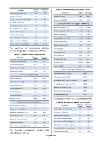
Results
With the above procedures executed, the
pseudocritical properties of natural gas are,
Table 6. Sutton Correlation & Wichert & Aziz
Correction
The upstream & downstream pipeline
mechanical design data is estimated as
follows,
Table 7. Pipeline Mechanical Design Results](https://image.slidesharecdn.com/naturalgastransmissiontutorial-191103080412/85/Process-Design-for-Natural-Gas-Transmission-10-320.jpg)
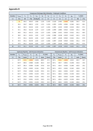
![Page 12 of 14
For the iterative steps made for compressor
discharge temperature [T2], Upstream &
Downstream Pipeline Exit Pressure [Pe]
calculations, the error percentage in the
iterative steps is plotted below.
Figure 2. Error Percentage in Iterative Steps
Appendix A shows a summary of the MS-
Excel Steps & Appendix B shows the
iterations made to calculate the compressor
discharge temperature [T2], Upstream &
Downstream Pipeline Exit Pressures [Pe].
References
1. “Handbook of Natural Gas Engineering”,
Katz, D.L., 1959, McGraw-Hill Higher
Education, New York
2. “Gases and Vapors At High Temperature
and Pressure - Density of Hydrocarbon”, Kay
W, 1936 Ind. Eng. Chem. 28 (9): 1014-1019
(http://dx.doi.org/10.1021/ie50321a008)
3. “Density of Natural Gases”, Standing, M.B.
and Katz, D.L. 1942 In Transactions of the
American Institute of Mining and
Metallurgical Engineers, No. 142, SPE-
942140-G, 140–149, New York
4. “Compressibility Factors for High-
Molecular-Weight Reservoir Gases”, Sutton,
R.P. 1985. SPE Annual Technical
Conference & Exhibition, Las Vegas,
Nevada, USA, 22-26 Sep, SPE-14265-MS
(http://dx.doi.org/10.2118/14265-MS)
5. “Calculation of Z Factors For Natural Gases
Using Equations of State”, Dranchuk, P.M.
and Abou-Kassem, H. 1975, J Can Pet
Technol 14 (3): 34. PETSOC-75-03-
03 (http://dx.doi.org/10.2118/75-03-03)
6. https://petrowiki.org/Real_gases
7. “Compressibility Factors for Naturally
Occurring Petroleum Gases, Piper, L.D.,
McCain Jr., W.D., and Corredor, J.H., SPE
Annual Technical Conference & Exhibition,
Houston, 3–6 October 1993, SPE-26668-
MS (http://dx.doi.org/10.2118/26668-MS)
8. “Handbook of Natural Gas Transmission and
Processing, Principles and Practices, Saied
Mokhatab, Wilaim A. Poe, John Y Mak, 3rd
Edition
9. “Pipeline Systems, Design, Construction,
Maintenance and Asset Management”,
Nandagopal N.S, Rev. 4
10. “Standard for Gas Transmission and
Distribution Piping Systems”, ANSI/ASME
Standard B31.8, 1999
11. Recommended Practice for Analysis, Design,
Installation, and Testing of Basic Surface
Safety Systems for Offshore Production
Facilities,” API RP14C, 7th Ed, 2001
12. “Isobaric specific heat capacity of natural
gas as a function of specific gravity, pressure
and temperature”, Lateef A. Kareema,
Tajudeen M. Iwalewa, James E. Omeke,
Journal of Natural Gas Science and
Engineering 19 (2014) 74-83](https://image.slidesharecdn.com/naturalgastransmissiontutorial-191103080412/85/Process-Design-for-Natural-Gas-Transmission-12-320.jpg)


This document provides an overview of the process design methodology for natural gas transmission from a gas plant to a city power station via a pipeline and booster compressor station. Key details include: - Natural gas composition and properties, pipeline lengths and specifications - Three part design methodology for the upstream pipeline, booster compressor, and downstream pipeline - Property estimation methods including Kay's rule, Sutton correlations, and Dranchuk-Abou-Kassem equation of state - Accounting for non-hydrocarbon gases like CO2 and H2S using Wichert & Aziz correlations The design process involves estimating pipeline parameters, mixture properties, pressure drops, temperatures and flows to safely transmit the natural gas while


