This document describes a methodology for estimating natural gas hydrate formation in pipelines. It presents an empirical approach using equations to model the pipeline temperature profile based on factors like operating pressure, temperature, heat transfer rate, and Joule-Thomson cooling effect. The methodology is applied to a case study of a 20km pipeline carrying natural gas. The results show the pipeline exit temperature remains above the hydrate formation temperature calculated along the pipeline length using established correlations, avoiding hydrate plug formation. In practice, heating the inlet gas or adding hydrate inhibitors can further increase this difference to improve safety.

1. Page 1 of 3
Empirical Approach to Hydrate Formation in Natural Gas Pipelines
Jayanthi Vijay Sarathy, M.E, CEng, MIChemE, Chartered Chemical Engineer, IChemE, UK
Natural Gas Pipelines often suffer from
production losses due to hydrate plugging.
For an effective hydrate plug to form, factors
can vary from pipeline operating pressure
and temperature, presence of water below its
dew point, extreme winter conditions & Joule
Thomson cooling. In the event hydrates form
in the pipeline section, their consequence
depends on how well the hydrates
agglomerate to grow and form a column. If
the pipeline section temperature is only at
par with the hydrate formation temperature,
the particles do no agglomerate; instead they
have to cross the metastable region which is
of the order of 50C to 60C, before hydrate
formation accelerates to block the pipeline.
Figure 1. P-T Hydrate Curve [1]
Although engineering softwares exist to
estimate pipeline process conditions and also
generate a P-T hydrate curve, the following
tutorial provides a guidance summary to
estimate the expected pipeline temperature
profile and the associated hydrate formation
temperatures.
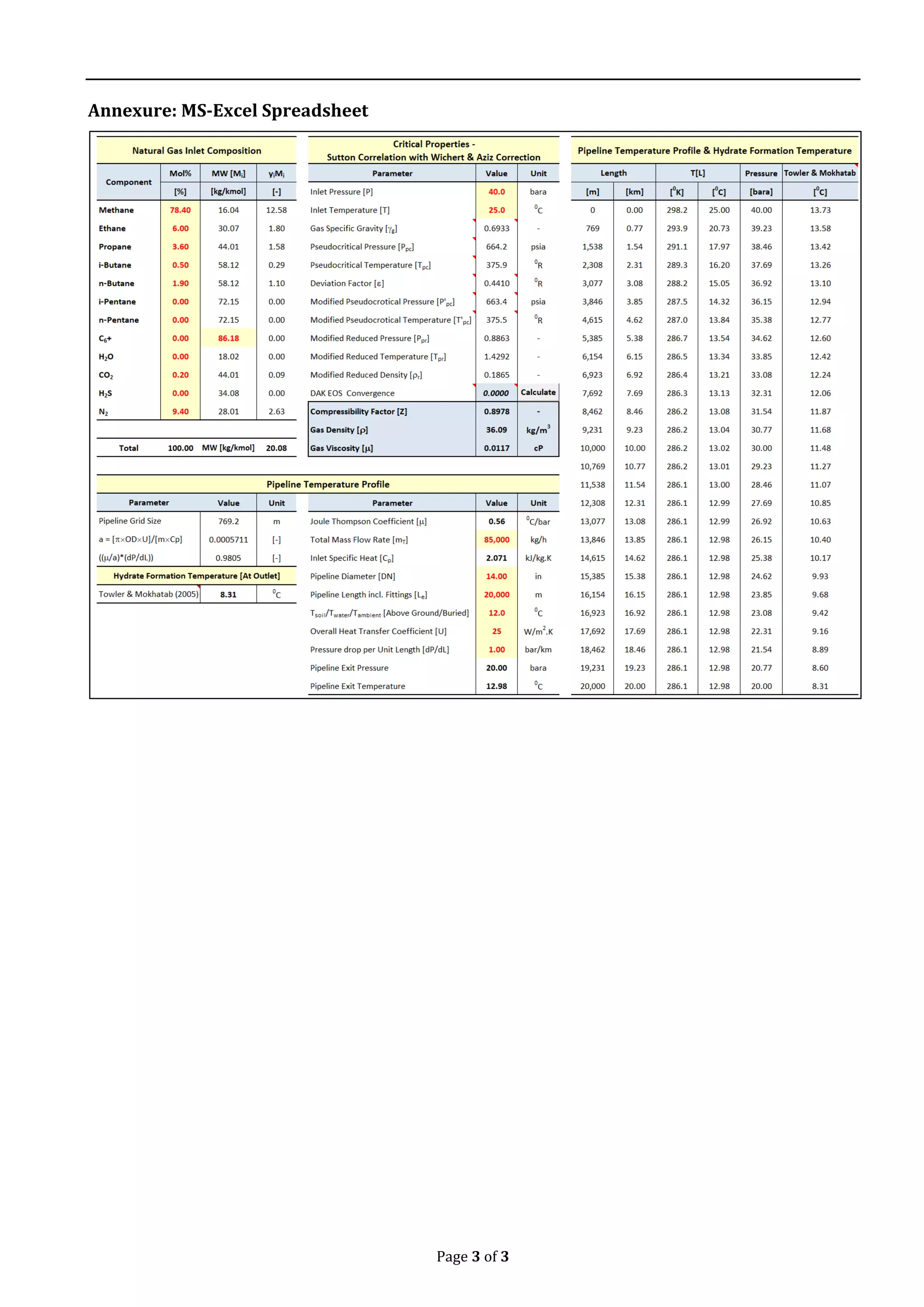
Problem Statement
A DN 14”, 20 km hydrocarbon line carrying
natural gas at the rate of 85,000 kg/h, 40 bara
and 250C is fed to a receiving station. The
total pipeline pressure drop per km [P/km]
is taken to be 1 bar/km. The overall heat
transfer coefficient is taken to be 25 W/m2.K.
The ambient temperature is 120C. The
hydrate formation temperature for the
composition is experimentally estimated to
be 500F at 325 psia. It is required to estimate
the pipeline exit temperature & the hydrate
formation temperature along the pipeline. For
the estimates, the Joule-Thomson coefficient
is assumed to be an average of 5.60C/bar
throughout the pipeline. The natural gas
composition is as follows,
Table 1. Gas Mixture [GPSA, Sec 20, Page 20-15]
Component
Mol% MW [Mi] yiMi
[%] [kg/kmol] [-]
Methane 78.40 16.04 12.58
Ethane 6.00 30.07 1.80
Propane 3.60 44.01 1.58
i-Butane 0.50 58.12 0.29
n-Butane 1.90 58.12 1.10
CO2 0.20 44.01 0.09
N2 9.40 28.01 2.63
Total 100.00 MW [kg/kmol] 20.08
Methodology
The pipeline temperature profile can be
estimated based on Coulter & Bardon (1979)
correlation [4]. The steady state temperature
profile is calculated from the momentum
equation, while omitting the potential &
kinetic energy terms in the enthalpy equation.
𝑑ℎ
𝑑𝐿
+
𝑑𝑄
𝑑𝐿
= 0 (1)
Where,
𝑄 =
𝜋×𝑂𝐷×𝑈×∆𝐿
𝑚
[𝑇0 − 𝑇𝑠] (2)
𝑑ℎ = 𝑐𝑝𝑑𝑇 − 𝜇𝑐𝑝𝑑𝑃 (3)
Where,

2. Page 2 of 3
U = Overall HTC [W/m2.K]
ID = Pipeline OD [m]
m = mass flow rate [kg/s]
L = Pipeline length [m]
T0 = Fluid Temperature [K]
Ts = Surrounding Temperature [K]
 = Joule-Thompson Coefficient [0C/bar]
Cp = Specific heat capacity [J/kg.K]
g = Gas Specific Gravity, MW/28.9625 [-]
Solving for pipeline temperature profile,
𝑇[𝐿] = [𝑇0 − 𝑇𝑠 − (
𝜇
𝑎
)(
𝑑𝑃
𝑑𝐿
)] 𝑒−𝑎𝐿
+ 𝑇𝑠 + (
𝜇
𝑎
) (
𝑑𝑃
𝑑𝐿
) (4)
Where,
𝑎 =
𝜋×𝑂𝐷×𝑈
𝑚×𝐶𝑝
It is to be noted that the specific heat [Cp] and
Joule-Thompson [J-T] co-efficient [] varies
with the pipeline pressure & temperature.
But for computational purposes, is assumed
to be constant. The purpose of including the J-
T coefficient is to account for cooling during
gas expansion along the pipeline. The ideal
mass specific heat [Cp], kJ/kg.K, of natural gas
can be computed as,
𝐶𝑝 = [(−10.9602𝛾𝑔 + 25.9033) + (0.21517𝛾𝑔 −
0.068687)𝑇 + (−0.00013337𝛾𝑔) + 0.000086387)𝑇2
+
(0.000000031474𝛾𝑔) − 0.000000028396)𝑇3
]/ 𝑀𝑊(5)
Where, T = Temperature [K]
Hydrate Formation Temperature
To estimate the hydrate formation
temperature [Th], Towler & Mokhatab (2005)
[3], proposed the following correlation,
𝑇ℎ[℉] = [13.47 × 𝑙𝑛(𝑃)] + [34.27 × 𝑙𝑛(𝛾)] −
[1.675 × 𝑙𝑛(𝑃) × 𝑙𝑛(𝛾)] − 20.35 (6)
Where,
P = Pressure [psia]
The validity of the above expression is for the
1. Temperature Range: 260 K to 298 K
2. Pressure Range: 1200 kPa to 40,000 kPa
3. MW: 16 g/mol to 29 g/mol (0.55 < g < 1.0)
Results
Substituting the values to arrive at the
pipeline temperature profile, the gas specific
gravity is estimated as,
𝛾𝑔 =
20.08
28.9625
= 0.6933 (7)
𝑎 =
𝜋×[
14×25.4
1000
]×25
[
85,000
3600
]×2.071×1000
= 0.0005711 (8)
𝑇[𝐿] = 12.0195 × 𝑒−0.0005711×𝐿
+ 286.1305 (9)
The hydrate formation temperature [Th] is,
𝑇ℎ[℉] = [14.0835 × 𝑙𝑛(𝑃, 𝑝𝑠𝑖)] − 32.9023 (10)
Plotting the above expressions, we get,
Figure 2. Hydrate Formation Temperature
From the plot, the pipeline temperature stays
above the hydrate formation temperature. In
practice, to increase the difference, the inlet
gas can be either heated or hydrate inhibitors
such as MeOH, MEG or TEG can be added.
References
1. https://www.sciencedirect.com/topics/en
gineering/hydrate-formation-curve
2. “Handbook of Natural gas Transmission and
Processing”, Saied Mokhatab, William A.
Poe, John Y. Mak, 3rd Edition.
3. “Hydrate Formation Calculation in the
Natural Gas Purification Unit”, J A Prajaka
et al 2019 IOP Conf. Ser.: Mater. Sci. Eng.
543 012084
4. Predicting Compositional Two Phase Flow
Behaviour in Pipelines, H. Furukawa, O.
Shoham, J.P. Brill, Transaction of the ASME,
Vol 108, September 1986.

3. Page 3 of 3
Annexure: MS-Excel Spreadsheet