The document discusses the generation and recycling of flash steam and steam condensates in power plant condensate return lines, outlining technical considerations for sizing and designing these lines. Key factors include the estimation of flash steam fractions, pressure drops, and the effects of gravity drainage, emphasizing the importance of proper design during various operational conditions. Additionally, it provides detailed calculations and guidelines for maintaining effective flow and preventing issues like water hammering.

1. Page 1 of 5
Flash Steam and Steam Condensates in Return Lines
Jayanthi Vijay Sarathy, M.E, CEng, MIChemE, Chartered Chemical Engineer, IChemE, UK
In power plants, boiler feed water is
subjected to heat thereby producing steam
which acts as a motive force for a steam
turbine. The steam upon doing work loses
energy to form condensate and is
recycled/returned back to reduce the
required make up boiler feed water (BFW).
Recycling steam condensate poses its own
challenges. Flash Steam is defined as steam
generated from steam condensate due to a
drop in pressure. When high pressure and
temperature condensate passes through
process elements such as steam traps or
pressure reducing valves to lose pressure, the
condensate flashes to form steam. Greater the
drop in pressure, greater is the flash steam
generated. This results in a two phase flow in
the condensate return lines
General Notes
1. To size condensate return lines, the
primary input data required to be
estimated is A. Fraction of Flash Steam and
condensate, B. Flow Rates of Flash Steam
& condensate, C. Specific volume of flash
steam & condensates, D. Velocity limits
across the condensate return lines.
2. Sizing condensate return lines also require
lower velocity limits for wet steam since
liquid droplets at higher velocities cause
internal erosion in pipes and excessive
piping vibration. A rule of thumb, for
saturated wet steam is 25 – 40 m/s for
short lines of the order of a few tens of
metres and 15 - 20 m/s for longer lines of
the order of a few hundred metres.
3. Condensate return lines work on the
principle of gravity draining. To effectuate
this, drain lines are to be sloped downward
at a ratio of atleast 1:100.
4. Proper sizing of stem condensate return
lines requires consideration of all
operating scenarios, chiefly start up,
shutdown and during normal running
conditions. During plant start up, steam is
not generated instantly. As a result, the
condensate lines would be filled with
liquids which gradually turn two-phase
until reaching normal running conditions.
During shutdown conditions, with time,
flash steam in the lines condense leaving
behind condensates due to natural cooling.
5. Condensate return line design must also
consider the effects of water hammering.
When multiple steam return lines are
connected to a header pipe that is routed
to a flash drum, flash steam in the presence
of cooler liquid from other streams would
condense rapidly to cause a water hammer.
Fraction of Flash Steam
Taking an example case, condensate flows
across a control valve from an upstream
pressure of 5 bara to 2 bara downstream. The
saturation temperature at 5 bara is 151.84 0C
& 120.20C at 2 bara. The specific volume of
water at 5 bara is 0.001093 m3/kg & 0.00106
m3/kg at 2 bara. The latent heat of saturated
steam upon reaching 2 bara is 2201.56 kJ/kg.
The % flash steam generated is estimated as,
ℎ𝑓,1 = ℎ𝑓,2 + [
% 𝐹𝑙𝑎𝑠ℎ
100
× ℎ𝑓𝑔] (1)
Where,
hf,1 = Upstream specific enthalpy [kJ/kg]
hf,2 = Downstream specific enthalpy [kJ/kg]
hf,g = Latent Heat of Saturated Steam [kJ/kg]
The upstream specific enthalpy, hf1 of
saturated water at 5 bara is 640.185 kJ/kg
and hf2 of 504.684 kJ/kg at 2 bara. The steam
specific volume at 2 bara is 0.8858 m3/kg.

2. Page 2 of 5
The fraction of flash steam is calculated as,
% 𝐹𝑙𝑎𝑠ℎ =
[640.185−504.684]
2201.56
× 100 = 6.15% (2)
Therefore the condensate fraction is,
% 𝐶𝑜𝑛𝑑 = 100 − 6.15 = 93.85% (3)
The steam volume is calculated as,
𝑉𝑆𝑡𝑒𝑎𝑚 = 0.8858 × 0.0615 = 0.05448
𝑚3
𝑘𝑔
(4)
The condensate volume is calculated as,
𝑉𝐶𝑜𝑛𝑑 = 0.00106 × 0.9385 = 0.000995
𝑚3
𝑘𝑔
(5)
Condensate Return Pipe Sizing
To size the condensate return line, the bulk
properties and mixture properties can be
used to estimate the pipe size. It must be
remembered that as the two-phase mixture
travels through the pipe, there is a pressure
profile that causes the flash % to change
along the pipe length. Additionally due to the
pipe inclination, a certain amount of static
head is added to the total pressure drop.
To estimate the pipe pressure drop across the
pipe length, a homogenous model for
modelling the two phase pressure drop can
be adopted. The homogenous mixture acts as
a pseudo-fluid, that obeys conventional
design based on single phase fluids
characterized by the fluid’s average
properties.
The mixture properties can be estimated as,
𝜌ℎ = 𝜌 𝐿[1 − 𝜀ℎ] + 𝜌 𝑣 𝜀ℎ (6)
Where,
L = Condensate Density [kg/m3]
v = Steam Density [kg/m3]
h = Homogenous void fraction for a given
steam quality [x] [-]
The homogenous void fraction [h] for a given
steam quality [x] can be estimated as,
𝜀ℎ =
1
1+[
𝑢 𝑣
𝑢 𝐿
×
1−𝑥
𝑥
×
𝜌 𝑣
𝜌 𝐿
]
(7)
The dynamic viscosity for calculating the
Reynolds number can be chosen as the
viscosity of the liquid phase or a quality
averaged viscosity, µh.
𝜇ℎ = 𝑥𝜇 𝑣 + [1 − 𝑥]𝜇 𝐿 (8)
The homogenous model for gravitational
pressure drop is applicable for large drop in
pressures and mass velocities < 2000
kg/m2.s, such that sufficient turbulence exists
to cause both phases to mix properly and
ensure the slip ratio (uv/uL) between the
vapour and liquid phase is ~1.0. For more
precise estimates capturing slip ratios and
varying void fraction, correlations such as
Friedal (1979), Chisholm (1973) or Muller-
Steinhagen & Heck (1986) can be used.
The total pressure drop is the sum of the
static head, frictional pressure drop &
pressure drop due to momentum pressure
gradient.
∆𝑃𝑇 = ∆𝑃𝑠𝑡𝑎𝑡𝑖𝑐 + ∆𝑃𝑚𝑜𝑚 + ∆𝑃𝑓𝑟𝑖𝑐 (9)
The Static Head [Pstatic] is computed as,
∆𝑃𝑠𝑡𝑎𝑡𝑖𝑐[𝑏𝑎𝑟] =
𝐻×𝜌ℎ× 𝑔×𝑆𝑖𝑛𝜃
105
(10)
Where,
H = Pipe Elevation [m]
 = Pipe inclination w.r.t horizontal [degrees]
The pressure drop due to momentum
pressure gradient [Pmom] is,
𝑑𝑃
𝑑𝑍
=
𝑑( 𝑚
𝜌ℎ⁄ )
𝑑𝑍
(11)
If the vapour fraction remains constant across
the piping, the pressure drop due to
momentum pressure gradient is negligible.
The frictional pressure drop is calculated as,
∆𝑃𝑓 =
𝑓×𝐿×𝜌ℎ×𝑉2
2𝐷
(12)
Where, P = Pressure drop [bar]
f =Darcy Friction Factor [-]

3. Page 3 of 5
L = Pipe Length [m]
h = Mixture Density [kg/m3]
V = Bulk fluid Velocity [m/s]
D = Pipe Inner Diameter, ID [m]
Re =
DVρh
µh
(13)
Where, µh = Dynamic Viscosity [kg.m/s]
h = Homogenous Density [kg/m3]
The Darcy Friction Factor [f] depends on the
Reynolds number follows the following
criteria,
If Re <= 2100 ; Hagen Poiseuille’s Equation
If Re <= 4000 ; Churchill Equation
If Re > 4000 ; Colebrook Equation
The Laminar Flow equation also referred to
as the Hagen Poiseuille’s equation is,
f =
64
Re
(14)
The Churchill equation combines both the
expressions for friction factor in both laminar
& turbulent flow regimes. It is accurate to
within the error of the data used to construct
the Moody diagram. This model also provides
an estimate for the intermediate (transition)
region; however this should be used with
caution.
The Churchill equation shows very good
agreement with the Darcy equation for
laminar flow, accuracy through the
transitional flow regime is unknown & in the
turbulent regime a difference of around 0.5-
2% is observed between the Churchill
equation and the Colebrook equation. For
Reynolds number up to ~4000,
f = 8 [(
8
Re
)
12
+
1
(A+B)1.5
]
1
12⁄
(15)
A = [2.457ln (
1
(
7
Re
)
0.9
+0.27
ε
D
)]
16
(16)
B = [(
37,530
Re
)]
16
(17)
The Colebrook equation was developed
taking into account experimental results for
the flow through both smooth and rough pipe.
It is valid only in the turbulent regime for
fluid filled pipes. Due to the implicit nature of
this equation it must be solved iteratively. A
result of suitable accuracy for almost all
industrial applications will be achieved in less
than 10 iterations. For Reynolds number up
greater than ~4000,
1
√f
= −2 log10 [
ε DH⁄
3.7
+
2.51
Re√f
] (18)
Homogenous Property Calculations
The two phase mixture flows through the
condensate return line. The associated
density and viscosity of flash steam and
condensate at 2 bara and 120.20C is,
𝜌 𝑣 =
1
0.8858
= 1.129
𝑘𝑔
𝑚3
(19)
𝜌 𝐿 =
1
0.00106
= 943.4
𝑘𝑔
𝑚3
(20)
𝜇 𝑣 = 0.000229
𝑘𝑔
𝑚.𝑠
(21)
𝜇 𝐿 = 0.0000128
𝑘𝑔
𝑚.𝑠
(22)
The homogenous void fraction [h] for a slip
ratio (uv/uL) of 1.0, i.e., uv = uL, and a steam
quality [x] of 6.15% is,
𝜀ℎ =
1
1+[1×
1−0.0615
0.0615
×
1.129
943.4
]
= 0.9821 (23)
The two phase homogeneous density is,
𝜌ℎ = 943.4 × [1 − 0.9821] + [1.129 × 0.9821] (24)
𝜌ℎ = 18.01
𝑘𝑔
𝑚3
(25)
The two phase homogeneous viscosity is,
𝜇ℎ =
0.0615×1.28
10−5
+
[1−0.9821]×2.29
10−4
(26)
𝜇ℎ = 0.000216
𝑘𝑔
𝑚.𝑠
(27)
Pressure Drop Calculations
The return condensate line from the control
valve discharge is sloped at a ratio of 1:100
for gravity drain. The layout of the return
condensate line is,

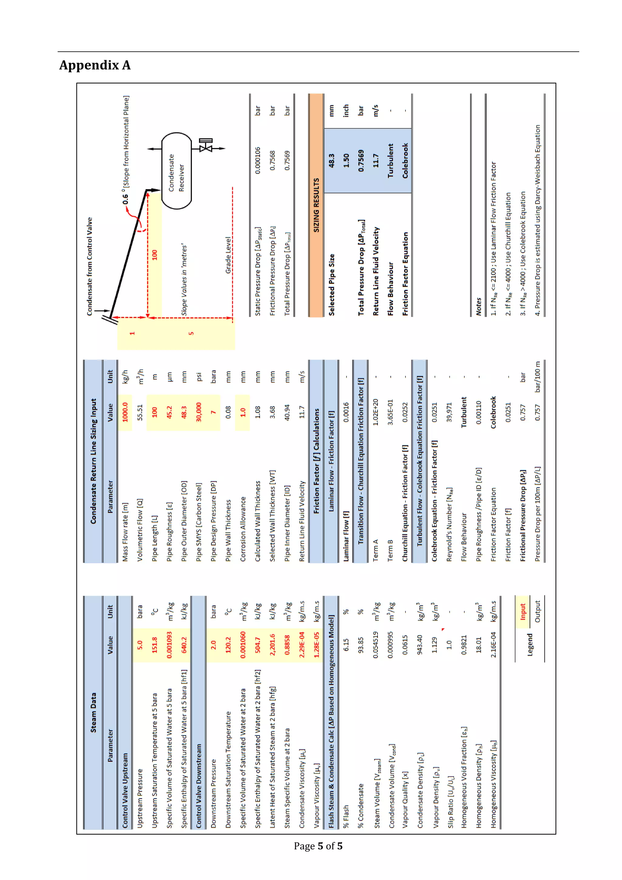
4. Page 4 of 5
Figure 1. Condensate Return Line to Receiver
The condensate receiver operates at 1.1 bara
pressure. The mechanical details of the piping
for a flow rate of 1,000 kg/h, pipe size of 1.5”,
100m length & pipe roughness of 45.2 m is,
Table 1. Condensate Return Line Details
Parameter Value Unit
Mass Flow rate [m] 1000.0 kg/h
Volumetric Flow [Q] 55.51 m3/h
Pipe Length [L] 100 m
Pipe Roughness [ε] 45.2 μm
Pipe Outer Diameter [OD] 48.3 mm
Pipe SMYS [Carbon Steel] 30,000 psi
Pipe Design Pressure [DP] 7 bara
Pipe Wall Thickness [WT] 0.08 mm
Corrosion Allowance [CA] 1.0 mm
Calculated WT 1.08 mm
Selected WT 3.68 mm
Pipe Inner Diameter [ID] 40.94 mm
The pipe wall thickness chosen is based on
ASME/ANSI B36.10M and is calculated based
on the hoop stress created by internal
pressure in a thin wall cylindrical vessel as,
WT =
DP×OD
2×SMYS
=
[7×14.5]×[
48.3
25.4
]
2×30,000
× 25.4 (28)
WT = 0.08𝑚𝑚 (29)
Adding CA of 1 mm, the WT becomes 1.08
mm. Based on ASME/ANSI B36.10M, the
selected WT is 3.68mm. The inner diameter
calculated for the selected WT is 40.94 mm.
The condensate return line mixture fluid
velocity is calculated as,
V =
Q
A
=
4×[
1000
18.01
]×
1
3,600
π×[0.04094]2
= 11.7 𝑚/𝑠 (30)
The Reynolds number is estimated as,
Re =
ID×V×𝜌ℎ
𝜇ℎ
=
0.04094×11.7×18.01
0.000216
(31)
Re = 39,971 (32)
Since the Reynolds number is much higher
than 4,000, the flow is fully turbulent and the
friction factor is calculated based on
Colebrook equation. The friction factor is
estimated as,
𝑓 = 𝑓𝐶𝑜𝑙𝑒𝑏𝑟𝑜𝑜𝑘 = 0.0251 (33)
The frictional pressure drop is now calculated
using the Darcy-Weisbach expression as,
∆𝑃𝑓 =
0.0251×100×18.01×11.72
2×0.04094×105
(34)
∆𝑃𝑓 = 0.757 𝑏𝑎𝑟 (35)
The slope angle is calculated as,
𝜃 = [𝑇𝑎𝑛−1
(
1
100
)] ×
180
𝜋
= 0.6° (36)
The static pressure drop [Pstatic] becomes
∆𝑃𝑠𝑡𝑎𝑡𝑖𝑐 =
18.01×9.81×[(1+5)×𝑠𝑖𝑛(0.6°)]
105
(37)
∆𝑃𝑠𝑡𝑎𝑡𝑖𝑐 = 0.000106 𝑏𝑎𝑟 (38)
Therefore the total P with negligible P due
to momentum pressure gradient [Pmom].
∆𝑃𝑡𝑜𝑡𝑎𝑙 = ∆𝑃𝑠𝑡𝑎𝑡𝑖𝑐 + ∆𝑃𝑓 (39)
∆𝑃𝑡𝑜𝑡𝑎𝑙 = 0.757 + 0.000106 = 0.757 𝑏𝑎𝑟 (40)
The condensate exit pressure is 2 – 0.757 =
1.243 bara which is higher than the receiver’s
operating pressure of 1.1 bara.
References
1. “Engineering Data Book III”, Ch 13, Two
Phase Pressure Drop, Wolverine Tube, Inc.
2. “Steam Handbook”, Dr. Ian Roberts, Philip
Stoor, Michael Carr, Dr. Rainer Hocker,
Oliver Seifert, Endress+Hauser

5. Page 5 of 5
Appendix A