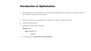
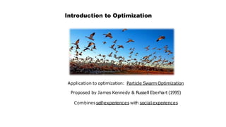
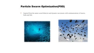
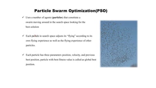
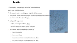
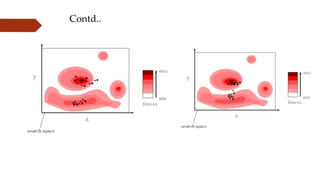
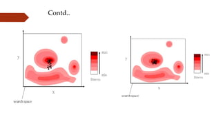
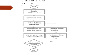
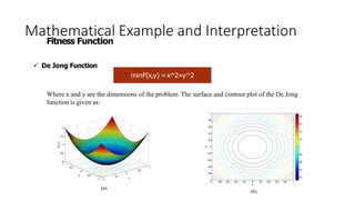
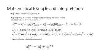
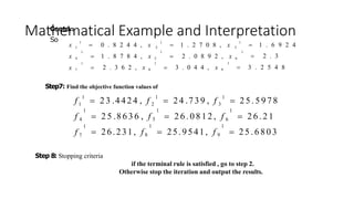
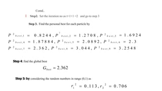
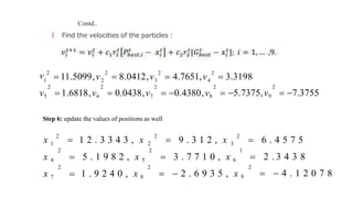
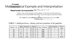
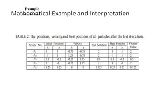
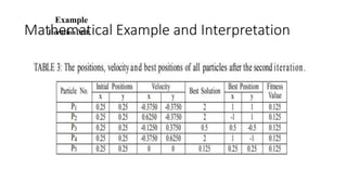
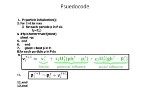
Particle Swarm optimization
Contents
 Introduction to Optimization
 Particle Swarm Optimization
 Illustration of Algorithm
 Mathematical Interpretation
 Example
 Dataset Illustration
Introduction to Optimization
🠶 The optimization can be defined as a mechanism through which the maximum or minimum value of a
given function or process can be found.
🠶 The function that we try to minimize or maximize is called as objective function.
🠶 Variable and parameters.
🠶 Statement of optimization problem
Minimize f(x)
subject to g(x)<=0
h(x)=0.
🠶 Two main phases Exploration and Exploitation
Introduction to Optimization
Application to optimization: Particle Swarm Optimization
Proposed by James Kennedy & Russell Eberhart (1995)
Combinesself-experiences with social experiences
Particle Swarm Optimization(PSO)
🠶 Inspired from the nature social behavior and dynamic movements with communications of insects,
birds and fish.
Particle Swarm Optimization(PSO)
 Uses a number of agents (particles) that constitute a
swarm moving around in the search space looking for the
best solution
 Each par🠶ticle in search space adjusts its “flying” according to its
own flying experience as well as the flying experience of other
particles.
 Each particle has three parameters position, velocity, and previous
best position, particle with best fitness value is called as global best
position.
Contd..
 Collection of flying particles (swarm) - Changing solutions
Search area - Possible solutions
 Movement towards a promising area to get the global optimum.
 Each particle adjusts its travelling speed dynamically corresponding to the flying
experiences of itself and its colleagues.
 Each particle keeps track:
its best solution, personal best, pbest.
the best value of any particle, global best, gbest.
 Each particle modifies its position according to:
• its current position
• its current velocity
• the distance between its current position and pbest.
• the distance between its current position and gbest.
Algorithm - Parameters
f : Objective function
Xi: Position of the particle or agent.
Vi: Velocity of the particle or agent.
A: Population of agents.
W: Inertia weight.
C1: cognitive constant.
R1, R2: random numbers.
C2: social constant.
Algorithm - Steps
1. Create a ‘population’of agents (particles) uniformly distributed over X
2. Evaluate each particle’s position according to the objective function( say
y=f(x)= -x^2+5x+20
1. If a particle’s current position is better than its previous best position, update it.
2. Determine the best particle (according to the particle’s previous best positions).
Y=F(x) =-x^2+5x+20
Contd..
5. Update particles’velocities:
6. Move particles to their new positions:
7. Go to step 2 until stopping criteria are satisfied.
Contd…
Particle’s velocity
:
1. Inertia
2. Personal
Influence
3. Social
Influence
• Makes the particle move in the same direction and
with the same velocity
• Improves the individual
• Makes the particle return to a previous position,
better than the current
• Conservative
• Makes the particle follow the best neighbors
direction
Acceleration coefficients
• When , c1=c2=0 then all particles continue flying at their current speed until they hit the search space’s boundary.
Therefore, the velocity update equation is calculated as:
t
 v i j
t  1
v i j
• When c1>0 and c2=0 , all particles are independent. The velocity update equation will be:
t  1
v i j
 v i j  c 1 r 1 j P b e s t , i  x 
t t t t
i j
• When c1>0 and c2=0 , all particles are attracted to a single point in the entire swarm and
the update velocity will become
g b e s t
 x i j 
t
t t
 v i j  c 2 r 2 j
t  1
v i j
• When c1=c2, all particles are attracted towards the average of pbest and gbest.
Contd…
 Intensification: explores the previous solutions, finds the best solution of a
given region
 Diversification: searches new solutions, finds the regions with potentially the
best solutions
 In PSO:

Example:
Contd..
Contd..
Contd..
Flow chart of
Algorithm
Mathematical Example and Interpretation
Fitness Function
 De Jong Function
minF(x,y) =x^2+y^2
Where x and y are the dimensions of the problem. The surface and contour plot of the De Jong
function is given as:
Mathematical Example and Interpretation
Contd..
Rastrigin Function
The surface and contour plot of the De Jong function is given as:
D
(xi 10.cos(2..xi )
t1
Mathematical Example and Interpretation
Contd…
Banana Function
The surface and contour plot of the Rosenbrock function or 2nd De Jong function
Or valley or banana functions given as:
Mathematical Example and Interpretation
  1 . 1 ,
f (x)   x2
 5x  20
Using PSO algorithm. Use 9 particles with initial positions
x 1   9 . 6 , x 2   6 , x 3   2 . 6 , x 4
x 5  0 . 6 , x 6  2 . 3 , x 7  2 . 8 , x 8  8 . 3 , x 9  1 0
Solution Choose the number of particles
x 1   9 . 6 , x 2   6 , x 3   2 . 6 , x 4   1 . 1 ,
x 5  0 . 6 , x 6  2 . 3 , x 7  2 . 8 , x 8  8 . 3 , x 9  1 0
Evaluate the objective function
0
  7 . 3 9 , f 9   3 0
0
 2 6 . 1 6 , f 8
0 0
 1 3 . 2 9 , f 5  2 2 . 6 4 , f 6  2 6 . 2 1 ,
0 0 0
f 1   1 2 0 . 1 6 , f 2   4 6 , f 3  0 . 2 4
0
f 4
0
f 7
Mathematical Example and Interpretation
0
9
0
8
0
7
0
6
5
0 0
1  0
 v
 v
 v
 v
 0, v 0
 v 0
, v 0
, v  v
1 2 3 4
v 0
Step2. Set the iteration no as t=0+1 and go to step 3
.
Step 3. Find the personal best for each particle by
So
  2 . 6
 2 . 3
 2 . 8 , P 1
b e s t , 8  8 . 3 , P 1
b e s t , 9  1 0
  6 , P 1
b e s t , 3
 0 . 6 , P 1
b e s t , 6
  9 . 6 , P 1
b e s t , 2
  1 . 1 , P 1
b e s t , 5
P 1
b e s t , 1
P 1
b e s t , 4
P 1
b e s t , 7
Mathematical Example and Interpretation
..
Step 4: Gbest =max(Pbest) so gbest =(2.3).
Step 5: updating the velocities of the particle by considering the value of random
numbers r1 = 0.213, r2= 0.876, c1=c2=1, w=1.
v 1
 00.213(9.69.6)0.876(2.39.6) 10.4244
1
1 1 1 1 1 1 1
v2  7.2708,v3  4.2924,v5 1.4892,v6  0,v7  0.4380,v8 5.256,v9  6.7452
Step 6: update the values of positions as well
Mathematical Example and Interpretation
Contd..
So 1
3
1
2
1
1
 3 . 2 5 4 8
 1 . 6 9 2 4
 2 . 3
1
 3 . 0 4 4 , x 9
1
 2 . 3 6 2 , x 8
1
 2 . 0 8 9 2 , x 6
1 1
x 4  1 . 8 7 8 4 , x 5
1
x 7
 1 . 2 7 0 8 , x
 0 . 8 2 4 4 , x
x
Step7: Find the objective function values of
1
3
1 1
1 2  2 5 . 5 9 7 8
1 1
 26.231, f 8  25.9541, f 9  2 5 . 6 8 0 3
1
 2 6 . 0 8 1 2 , f 6  2 6 . 2 1
1 1
f 4  2 5 .8 6 3 6 , f 5
1
f 7
 2 4 .7 3 9 , f
 2 3 .4 4 2 4 , f
f
Step 8: Stopping criteria
if the terminal rule is satisfied , go to step 2.
Otherwise stop the iteration and output the results.
 1 . 6 9 2 4
 1 . 8 7 8 8 4 , P 2
b e s t , 5  2 . 0 8 9 2 , P 2
b e s t , 6  2 . 3
 2 . 3 6 2 , P 2
b e s t , 8  3 . 0 4 4 , P 2
b e s t , 9  3 . 2 5 4 8
Contd..
🠶 Step2. Set the iteration no as t=1+1 =2 and go to step 3
Step 3. Find the personal best for each particle by
2
 0 . 8 2 4 4 , P b e s t , 2  1 . 2 7 0 8 , P 2
b e s t , 3
P 2
b e s t ,1
P 2
b e s t , 4
P 2
b e s t , 7
 2.362
Step 4:find the global best
Gbest
Step 5: by considering the random numbers in range (0,1) as
2
2
1  0 . 7 0 6
 0 .11 3 , r
r 2
Contd..
🠶 Find the velocities of the particles :
2
2 2
2 3 4  3.3198
2
 5.7375,v9  7.3755
1
2 2 2 2
v5  1.6818,v6  0.0438,v7  0.4380,v8
 8.0412,v  4.7651,v
 11.5099,v
v 2
Step 6: update the values of positions as well
2
3
2
2 2
1
  4 . 1 2 0 7 8
 6 . 4 5 7 5
 2 . 3 4 3 8
2
  2 . 6 9 3 5 , x 9
1
 3 . 7 7 1 0 , x 6
2 2
x 4  5 . 1 9 8 2 , x 5
2 2
x 7  1 . 9 2 4 0 , x 8
 9 . 3 1 2 , x
 1 2 . 3 3 4 3 , x
x
Contd…
🠶 Step7: Find the objective function values of
 2 6 . 2 2 5 6
  1 7 . 5 8 3 9
2
 2 4 . 6 3 4 6 , f 6
2
  0 . 7 2 2 4 , f 9
2
 1 8 . 9 6 9 6 , f 5
2
 2 5 . 9 1 8 2 , f 8
2 2 2
f 1   7 0 . 4 6 4 4 , f 2   2 0 . 1 5 3 2 , f 3  1 0 . 5 8 8 2
2
f 4
2
f 7
Step 8: Stopping criteria
if the terminal rule is satisfied , go to step 2.
Otherwise stop the iteration and output the results
Contd..
🠶 Step2. Set the iteration no as t=1+2 =3 and go to step 3
Step 3. Find the personal best for each particle by
 1 . 6 9 2 4
 2 . 3 6 2 , P 3
b e s t , 8  3 . 0 4 4 , P 3
b e s t , 9  3 . 2 5 4 8
 1 . 8 7 8 8 4 , P 3
b e s t , 5  2 . 0 8 9 2 , P 3
b e s t , 6  2 . 3
 1 . 2 7 0 8 , P 3
b e s t , 3
 0 . 8 2 4 4 , P 3
b e s t ,
2
P 3
b e s t ,1
P 3
b e s t , 4
P 3
b e s t , 7
Step 4:find the global best
 2.362
Gbest
Step 5: by considering the random numbers in range (0,1) as
3
2
1  0 . 5 0 7
 0 .1 7 8 , r
r 3
Find the velocities of the particles
3 3
2 3 4  1.2909
3
 2.1531,v9  2.7759
1
3 3 3 3
v5  0.6681,v6  0.053,v7  0.1380,v8
 3.0862,v 3
 1.8405,v
 4.4052,v
v 3
Step 6: update the values of positions as well
3
3
2
3 3
1
 2 . 3 9 6 8
  6 . 8 9 6 7
 8 . 2 9 8
3
  4 . 8 4 6 6 , x 9
3
 1 . 7 8 6 , x 8
3 3
x 4  6 . 4 8 6 2 , x 5
3
x 7
 1 2 . 3 9 8 2 , x
3
 4 . 4 3 9 1 , x 6
 1 6 . 7 3 9 5 , x
x
Step7: Find the objective function values of
Contd..
• 3 3 3
• f 1   1 7 6 . 5 1 4 5 , f 2   7 1 . 7 2 4 4 , f 3   7 . 3 6 7 3
• 3
• f 4
• 3
• f 7
3
 2 2 . 4 9 , f 6  2 6 . . 2 3 9 3
  2 7 . 7 2 2 2 , f 3
  6 2 . 0 4 7 1
9
3
 1 0 . 3 3 6 7 , f 5
3
 2 5 . 7 4 0 2 , f 8
Step 8: Stopping criteria
if the terminal rule is satisfied , go to step 2.
Otherwise stop the iteration and output the results
Mathematical Example and Interpretation
 y2
Fitness Function :De Jong function min F (x, y) x2
Where x and y are the dimensions of the problem , the velocities of all the particles are
initialized to zero and inertia (W) = 0.3, and the value of the cognitive and social constants
are
C1= 2 and C2 =2. The initial best solutions of all the particles are set to 1000
Example
Iteration First:
P1 fitness value = 1 2
 1 2
 2
Mathematical Example and Interpretation
Example
Iteration 2nd:
Mathematical Example and Interpretation
Example
Iteration 3rd:
Mathematical Example and Interpretation
Example
Iteration 3rd:
Psuedocode
1. P=particle initialization();
2. For I=1to max
3 for each particle p in P do
fp=f(p)
4. Iffp is better than f(pbest)
pbest =p;
5. end
6. end
7. gbest =best p in P.
8.for each particle p in P do
9.
10.
11.end
12.end
DataSet
Advantages and Disadvantages of PSO
Advantages
 Insensitive to scaling of design variables.
 Simple implementation.
 Easily parallelized for concurrent processing.
 Derivative free.
 Very few algorithm parameters.
 Very efficient global search algorithm.
Disadvantages
 Slow convergence in refined search stage (weak local
search ability).

PSOPPT with example (pso optimization with solved problem) .pptx

  • 1.
  • 2.
    Contents  Introduction toOptimization  Particle Swarm Optimization  Illustration of Algorithm  Mathematical Interpretation  Example  Dataset Illustration
  • 3.
    Introduction to Optimization 🠶The optimization can be defined as a mechanism through which the maximum or minimum value of a given function or process can be found. 🠶 The function that we try to minimize or maximize is called as objective function. 🠶 Variable and parameters. 🠶 Statement of optimization problem Minimize f(x) subject to g(x)<=0 h(x)=0. 🠶 Two main phases Exploration and Exploitation
  • 4.
    Introduction to Optimization Applicationto optimization: Particle Swarm Optimization Proposed by James Kennedy & Russell Eberhart (1995) Combinesself-experiences with social experiences
  • 5.
    Particle Swarm Optimization(PSO) 🠶Inspired from the nature social behavior and dynamic movements with communications of insects, birds and fish.
  • 6.
    Particle Swarm Optimization(PSO) Uses a number of agents (particles) that constitute a swarm moving around in the search space looking for the best solution  Each par🠶ticle in search space adjusts its “flying” according to its own flying experience as well as the flying experience of other particles.  Each particle has three parameters position, velocity, and previous best position, particle with best fitness value is called as global best position.
  • 7.
    Contd..  Collection offlying particles (swarm) - Changing solutions Search area - Possible solutions  Movement towards a promising area to get the global optimum.  Each particle adjusts its travelling speed dynamically corresponding to the flying experiences of itself and its colleagues.  Each particle keeps track: its best solution, personal best, pbest. the best value of any particle, global best, gbest.  Each particle modifies its position according to: • its current position • its current velocity • the distance between its current position and pbest. • the distance between its current position and gbest.
  • 8.
    Algorithm - Parameters f: Objective function Xi: Position of the particle or agent. Vi: Velocity of the particle or agent. A: Population of agents. W: Inertia weight. C1: cognitive constant. R1, R2: random numbers. C2: social constant.
  • 9.
    Algorithm - Steps 1.Create a ‘population’of agents (particles) uniformly distributed over X 2. Evaluate each particle’s position according to the objective function( say y=f(x)= -x^2+5x+20 1. If a particle’s current position is better than its previous best position, update it. 2. Determine the best particle (according to the particle’s previous best positions). Y=F(x) =-x^2+5x+20
  • 10.
    Contd.. 5. Update particles’velocities: 6.Move particles to their new positions: 7. Go to step 2 until stopping criteria are satisfied.
  • 11.
    Contd… Particle’s velocity : 1. Inertia 2.Personal Influence 3. Social Influence • Makes the particle move in the same direction and with the same velocity • Improves the individual • Makes the particle return to a previous position, better than the current • Conservative • Makes the particle follow the best neighbors direction
  • 12.
    Acceleration coefficients • When, c1=c2=0 then all particles continue flying at their current speed until they hit the search space’s boundary. Therefore, the velocity update equation is calculated as: t  v i j t  1 v i j • When c1>0 and c2=0 , all particles are independent. The velocity update equation will be: t  1 v i j  v i j  c 1 r 1 j P b e s t , i  x  t t t t i j • When c1>0 and c2=0 , all particles are attracted to a single point in the entire swarm and the update velocity will become g b e s t  x i j  t t t  v i j  c 2 r 2 j t  1 v i j • When c1=c2, all particles are attracted towards the average of pbest and gbest.
  • 13.
    Contd…  Intensification: exploresthe previous solutions, finds the best solution of a given region  Diversification: searches new solutions, finds the regions with potentially the best solutions  In PSO: 
  • 14.
  • 15.
  • 16.
  • 17.
  • 18.
  • 19.
    Mathematical Example andInterpretation Fitness Function  De Jong Function minF(x,y) =x^2+y^2 Where x and y are the dimensions of the problem. The surface and contour plot of the De Jong function is given as:
  • 20.
    Mathematical Example andInterpretation Contd.. Rastrigin Function The surface and contour plot of the De Jong function is given as: D (xi 10.cos(2..xi ) t1
  • 21.
    Mathematical Example andInterpretation Contd… Banana Function The surface and contour plot of the Rosenbrock function or 2nd De Jong function Or valley or banana functions given as:
  • 22.
    Mathematical Example andInterpretation   1 . 1 , f (x)   x2  5x  20 Using PSO algorithm. Use 9 particles with initial positions x 1   9 . 6 , x 2   6 , x 3   2 . 6 , x 4 x 5  0 . 6 , x 6  2 . 3 , x 7  2 . 8 , x 8  8 . 3 , x 9  1 0 Solution Choose the number of particles x 1   9 . 6 , x 2   6 , x 3   2 . 6 , x 4   1 . 1 , x 5  0 . 6 , x 6  2 . 3 , x 7  2 . 8 , x 8  8 . 3 , x 9  1 0 Evaluate the objective function 0   7 . 3 9 , f 9   3 0 0  2 6 . 1 6 , f 8 0 0  1 3 . 2 9 , f 5  2 2 . 6 4 , f 6  2 6 . 2 1 , 0 0 0 f 1   1 2 0 . 1 6 , f 2   4 6 , f 3  0 . 2 4 0 f 4 0 f 7
  • 23.
    Mathematical Example andInterpretation 0 9 0 8 0 7 0 6 5 0 0 1  0  v  v  v  v  0, v 0  v 0 , v 0 , v  v 1 2 3 4 v 0 Step2. Set the iteration no as t=0+1 and go to step 3 . Step 3. Find the personal best for each particle by So   2 . 6  2 . 3  2 . 8 , P 1 b e s t , 8  8 . 3 , P 1 b e s t , 9  1 0   6 , P 1 b e s t , 3  0 . 6 , P 1 b e s t , 6   9 . 6 , P 1 b e s t , 2   1 . 1 , P 1 b e s t , 5 P 1 b e s t , 1 P 1 b e s t , 4 P 1 b e s t , 7
  • 24.
    Mathematical Example andInterpretation .. Step 4: Gbest =max(Pbest) so gbest =(2.3). Step 5: updating the velocities of the particle by considering the value of random numbers r1 = 0.213, r2= 0.876, c1=c2=1, w=1. v 1  00.213(9.69.6)0.876(2.39.6) 10.4244 1 1 1 1 1 1 1 1 v2  7.2708,v3  4.2924,v5 1.4892,v6  0,v7  0.4380,v8 5.256,v9  6.7452 Step 6: update the values of positions as well
  • 25.
    Mathematical Example andInterpretation Contd.. So 1 3 1 2 1 1  3 . 2 5 4 8  1 . 6 9 2 4  2 . 3 1  3 . 0 4 4 , x 9 1  2 . 3 6 2 , x 8 1  2 . 0 8 9 2 , x 6 1 1 x 4  1 . 8 7 8 4 , x 5 1 x 7  1 . 2 7 0 8 , x  0 . 8 2 4 4 , x x Step7: Find the objective function values of 1 3 1 1 1 2  2 5 . 5 9 7 8 1 1  26.231, f 8  25.9541, f 9  2 5 . 6 8 0 3 1  2 6 . 0 8 1 2 , f 6  2 6 . 2 1 1 1 f 4  2 5 .8 6 3 6 , f 5 1 f 7  2 4 .7 3 9 , f  2 3 .4 4 2 4 , f f Step 8: Stopping criteria if the terminal rule is satisfied , go to step 2. Otherwise stop the iteration and output the results.
  • 26.
     1 .6 9 2 4  1 . 8 7 8 8 4 , P 2 b e s t , 5  2 . 0 8 9 2 , P 2 b e s t , 6  2 . 3  2 . 3 6 2 , P 2 b e s t , 8  3 . 0 4 4 , P 2 b e s t , 9  3 . 2 5 4 8 Contd.. 🠶 Step2. Set the iteration no as t=1+1 =2 and go to step 3 Step 3. Find the personal best for each particle by 2  0 . 8 2 4 4 , P b e s t , 2  1 . 2 7 0 8 , P 2 b e s t , 3 P 2 b e s t ,1 P 2 b e s t , 4 P 2 b e s t , 7  2.362 Step 4:find the global best Gbest Step 5: by considering the random numbers in range (0,1) as 2 2 1  0 . 7 0 6  0 .11 3 , r r 2
  • 27.
    Contd.. 🠶 Find thevelocities of the particles : 2 2 2 2 3 4  3.3198 2  5.7375,v9  7.3755 1 2 2 2 2 v5  1.6818,v6  0.0438,v7  0.4380,v8  8.0412,v  4.7651,v  11.5099,v v 2 Step 6: update the values of positions as well 2 3 2 2 2 1   4 . 1 2 0 7 8  6 . 4 5 7 5  2 . 3 4 3 8 2   2 . 6 9 3 5 , x 9 1  3 . 7 7 1 0 , x 6 2 2 x 4  5 . 1 9 8 2 , x 5 2 2 x 7  1 . 9 2 4 0 , x 8  9 . 3 1 2 , x  1 2 . 3 3 4 3 , x x
  • 28.
    Contd… 🠶 Step7: Findthe objective function values of  2 6 . 2 2 5 6   1 7 . 5 8 3 9 2  2 4 . 6 3 4 6 , f 6 2   0 . 7 2 2 4 , f 9 2  1 8 . 9 6 9 6 , f 5 2  2 5 . 9 1 8 2 , f 8 2 2 2 f 1   7 0 . 4 6 4 4 , f 2   2 0 . 1 5 3 2 , f 3  1 0 . 5 8 8 2 2 f 4 2 f 7 Step 8: Stopping criteria if the terminal rule is satisfied , go to step 2. Otherwise stop the iteration and output the results
  • 29.
    Contd.. 🠶 Step2. Setthe iteration no as t=1+2 =3 and go to step 3 Step 3. Find the personal best for each particle by  1 . 6 9 2 4  2 . 3 6 2 , P 3 b e s t , 8  3 . 0 4 4 , P 3 b e s t , 9  3 . 2 5 4 8  1 . 8 7 8 8 4 , P 3 b e s t , 5  2 . 0 8 9 2 , P 3 b e s t , 6  2 . 3  1 . 2 7 0 8 , P 3 b e s t , 3  0 . 8 2 4 4 , P 3 b e s t , 2 P 3 b e s t ,1 P 3 b e s t , 4 P 3 b e s t , 7 Step 4:find the global best  2.362 Gbest Step 5: by considering the random numbers in range (0,1) as 3 2 1  0 . 5 0 7  0 .1 7 8 , r r 3
  • 30.
    Find the velocitiesof the particles 3 3 2 3 4  1.2909 3  2.1531,v9  2.7759 1 3 3 3 3 v5  0.6681,v6  0.053,v7  0.1380,v8  3.0862,v 3  1.8405,v  4.4052,v v 3 Step 6: update the values of positions as well 3 3 2 3 3 1  2 . 3 9 6 8   6 . 8 9 6 7  8 . 2 9 8 3   4 . 8 4 6 6 , x 9 3  1 . 7 8 6 , x 8 3 3 x 4  6 . 4 8 6 2 , x 5 3 x 7  1 2 . 3 9 8 2 , x 3  4 . 4 3 9 1 , x 6  1 6 . 7 3 9 5 , x x Step7: Find the objective function values of
  • 31.
    Contd.. • 3 33 • f 1   1 7 6 . 5 1 4 5 , f 2   7 1 . 7 2 4 4 , f 3   7 . 3 6 7 3 • 3 • f 4 • 3 • f 7 3  2 2 . 4 9 , f 6  2 6 . . 2 3 9 3   2 7 . 7 2 2 2 , f 3   6 2 . 0 4 7 1 9 3  1 0 . 3 3 6 7 , f 5 3  2 5 . 7 4 0 2 , f 8 Step 8: Stopping criteria if the terminal rule is satisfied , go to step 2. Otherwise stop the iteration and output the results
  • 32.
    Mathematical Example andInterpretation  y2 Fitness Function :De Jong function min F (x, y) x2 Where x and y are the dimensions of the problem , the velocities of all the particles are initialized to zero and inertia (W) = 0.3, and the value of the cognitive and social constants are C1= 2 and C2 =2. The initial best solutions of all the particles are set to 1000 Example Iteration First: P1 fitness value = 1 2  1 2  2
  • 33.
    Mathematical Example andInterpretation Example Iteration 2nd:
  • 34.
    Mathematical Example andInterpretation Example Iteration 3rd:
  • 35.
    Mathematical Example andInterpretation Example Iteration 3rd:
  • 36.
    Psuedocode 1. P=particle initialization(); 2.For I=1to max 3 for each particle p in P do fp=f(p) 4. Iffp is better than f(pbest) pbest =p; 5. end 6. end 7. gbest =best p in P. 8.for each particle p in P do 9. 10. 11.end 12.end
  • 37.
  • 38.
    Advantages and Disadvantagesof PSO Advantages  Insensitive to scaling of design variables.  Simple implementation.  Easily parallelized for concurrent processing.  Derivative free.  Very few algorithm parameters.  Very efficient global search algorithm. Disadvantages  Slow convergence in refined search stage (weak local search ability).