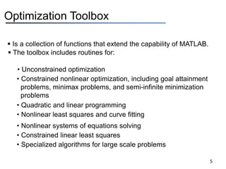
This document discusses optimization techniques in MATLAB. It describes how to perform both unconstrained and constrained optimization. For unconstrained problems, the fminunc function is used to find the minimum of an objective function. For constrained problems, fmincon is used to minimize an objective function subject to inequality, equality, and bound constraints. The document provides an example of using these functions to solve a sample constrained optimization problem.

1. Optimization with MATLAB
1

2.  Constraints
• Inequality
• Equality
Fundamentals of Non-Linear Optimization
 Single Objective function f(x)
• Maximization
• Minimization
 Design Variables, xi , i=0,1,2,3…..
Figure Example of design variables and
constraints used in non-linear optimization.
Maximize X1 + 1.5 X2
Subject to:
X1 + X2 ≤ 150
0.25 X1 + 0.5 X2 ≤ 50
X1 ≥ 50
X2 ≥ 25
X1 ≥0, X2 ≥0
 Optimal points
• Local minima/maxima points: A point or Solution x* is at local point
if there is no other x in its Neighborhood less than x*
• Global minima/maxima points: A point or Solution x** is at global
point if there is no other x in entire search space less than x**
2

3. Function Optimization
 Optimization concerns the minimization or maximization of
functions
 Standard Optimization Problem:
 
~
~
min
x
f x
 
~
0
j
g x 
 
~
0
i
h x 
L U
k k k
x x x
 
Equality Constraints
Subject to:
Inequality Constraints
Side Constraints
 
~
f x is the objective function, which measure and evaluate the performance of a
system. In a standard problem, we are minimizing the function. For
maximization, it is equivalent to minimization of the –ve of the objective
function.
Where:
~
x is a column vector of design variables, which can
affect the performance of the system.
3

4. Function Optimization (Cont.)
 
~
0
i
h x 
L U
k k k
x x x
 
Equality Constraints
Inequality Constraints
Side Constraints
 
~
0
j
g x 
Most algorithm require less than!!!
 Constraints – Limitation to the design space. Can be linear or
nonlinear, explicit or implicit functions
4

5. Optimization Toolbox
 Is a collection of functions that extend the capability of MATLAB.
 The toolbox includes routines for:
• Unconstrained optimization
• Constrained nonlinear optimization, including goal attainment
problems, minimax problems, and semi-infinite minimization
problems
• Quadratic and linear programming
• Nonlinear least squares and curve fitting
• Nonlinear systems of equations solving
• Constrained linear least squares
• Specialized algorithms for large scale problems
5

6. Unconstrained Minimization
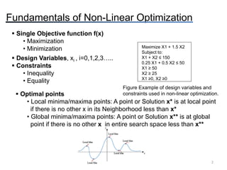
 Consider the problem of finding a set of values [x1 x2]T that
solves
   
1
~
2 2
1 2 1 2 2
~
min 4 2 4 2 1
x
x
f x e x x x x x
    
 Steps:
• Create an M-file that returns the function value (Objective
Function). Call it objfun.m
• Then, invoke the unconstrained minimization routine. Use fminunc
6
Example:
Solution:
Solve the following problem using optimtool ?

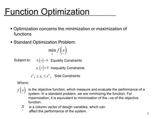
7. Step 1 – Obj. Function
function f = objfun(x)
f=exp(x(1))*(4*x(1)^2+2*x(2)^2+4*x(1)*x(2)+2*x(2)+1);
7
Step 2 – Invoke Routine
x0 = [-1,1];
[xmin,feval]=fminunc(‘objfun’,x0);

8. xmin =
0.5000 -1.0000
feval =
1.3028e-010
Minimum point of design variables
Objective function value
Results
8

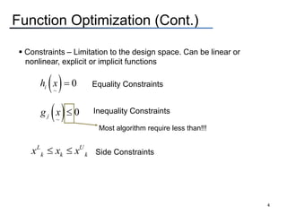
9. [xmin,feval,exitflag,output,lambda,grad,hessian] =
fmincon(fun,x0,A,B,Aeq,Beq,LB,UB,NONLCON,options,P1,P2,…)
Constrained Minimization
9

10.  
~
1 2 3
~
min
x
f x x x x
 
2
1 2
2 0
x x
 
1 2 3
1 2 3
2 2 0
2 2 72
x x x
x x x
   
  
1 2 3
0 , , 30
x x x
 
Subject to:
Example
10
Example: Solve the following problem using optimtool ?

11. 2
1 2
2 0
x x
 
For
Create a function call nonlcon which returns 2 constraint vectors [C,Ceq]
function [C,Ceq]=nonlcon(x)
C=2*x(1)^2+x(2);
Ceq=[];
Remember to return a null
Matrix if the constraint does
not apply
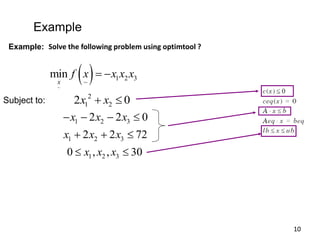
Solution:
11
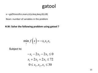
function f = myfun(x)
f=-x(1)*x(2)*x(3);

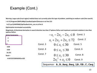
12. x0=[10;10;10];
A=[-1 -2 -2;1 2 2];
B=[0 72]';
LB = [0 0 0]';
UB = [30 30 30]';
[x,feval]=fmincon(@myfun,x0,A,B,[],[],LB,UB,@nonl
con)
1 2 2 0
,
1 2 2 72
A B
  
   
 
   
   
CAREFUL!!!
fmincon(fun,x0,A,B,Aeq,Beq,LB,UB,NONLCON,options,P1,P2
,…)
0 30
0 , 30
0 30
LB UB
   
   
 
   
   
   
Example (Cont.)
12

13. Warning: Large-scale (trust region) method does not currently solve this type of problem, switching to medium-scale (line search).
> In D:ProgramsMATLAB6p1toolboxoptimfmincon.m at line 213
In D:usrCHINTANGOptToolboxmin_con.m at line 6
Optimization terminated successfully:
Magnitude of directional derivative in search direction less than 2*options.TolFun and maximum constraint violation is less than
options.TolCon
Active Constraints:
2
9
x =
0.00
0.00
16.231
feval =
-4.657237250542452e-025 2
1 2
2 0
x x
 
1 2 3
1 2 3
2 2 0
2 2 72
x x x
x x x
   
  
1
2
3
0 30
0 30
0 30
x
x
x
 
 
 
Const. 1
Const. 2
Const. 3
Const. 4
Const. 5
Const. 6
Const. 7
Sequence: A,B,Aeq,Beq,LB,UB,C,Ceq
Const. 8
Const. 9
Example (Cont.)
13

14. >> optimtool - % GUI
14

15. gatool
x = ga(fitnessfcn,nvars,A,b,Aeq,beq,LB,UB)
Nvars :number of variables in the problem
H.W: Solve the following problem using gatool ?
15
 
~
1 2 3
~
min
x
f x x x x
 
1 2 3
1 2 3
2 2 0
2 2 72
x x x
x x x
   
  
1 2 3
0 , , 30
x x x
 
Subject to: