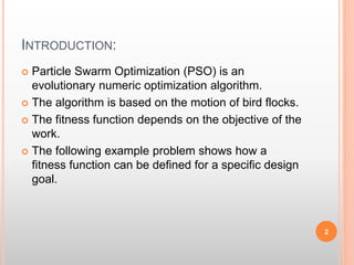
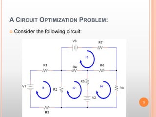
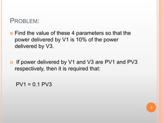
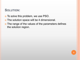
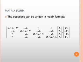
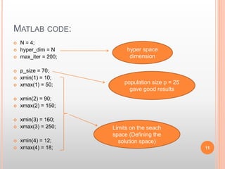
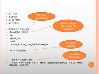
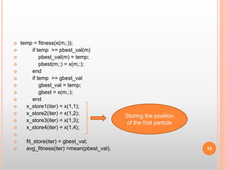
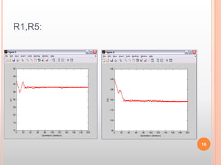
Particle swarm optimization is used to optimize circuit parameters to meet a specific design goal. The algorithm models the movement of bird flocks. It defines a fitness function that is maximized to find the optimal values of four circuit parameters (R1, R5, R8, V3) such that the power from voltage source V1 is 10% of the power from V3. The circuit equations are set up and solved using mesh current analysis. PSO runs for multiple iterations, updating particle velocities and positions to find the parameter values that maximize fitness.

1. PARTICLE SWARM OPTIMIZATION
1

2. INTRODUCTION:
 Particle Swarm Optimization (PSO) is an
evolutionary numeric optimization algorithm.
 The algorithm is based on the motion of bird flocks.
 The fitness function depends on the objective of the
work.
 The following example problem shows how a
fitness function can be defined for a specific design
goal.
2

3. A CIRCUIT OPTIMIZATION PROBLEM:
 Consider the following circuit:
3

4. CIRCUIT PARAMETERS:
 The circuit parameters have the following values:
R2 = 100Ω
R3 = 47Ω
R4 = 32Ω
R6 = 22Ω
R7 = 132Ω
V1 = 8 volt
V2 = 12 volt
 The other circuit parameters are variables. The range of
values of those parameters are:
R1 = 10Ω to 50Ω
R5 = 90Ω to 150Ω
R8 = 160Ω to 250Ω
v3 = 12 volt to 18 volt 4

5. PROBLEM:
 Find the value of these 4 parameters so that the
power delivered by V1 is 10% of the power
delivered by V3.
 If power delivered by V1 and V3 are PV1 and PV3
respectively, then it is required that:
PV1 = 0.1 PV3
5

6. SOLUTION:
 To solve this problem, we use PSO.
 The solution space will be 4 dimensional.
 The range of the values of the parameters defines
the solution region.
6

7. MESH EQUATIONS:
 First we need to find the power delivered by the
sources by solving the circuit.
 We use Mesh current analysis.
 The mesh equations are:

7
 
 
 
  VRIRRRIRI
VRIRRRIRI
VRIRIRRRIRI
VRIRRRI
263865452
364764342
25443542221
1223211





8. MATRIX FORM:
 The equations can be written in matrix form as:
8





















































V
V
V
V
I
I
I
I
RRRRR
RRRRR
RRRRRR
RRRR
2
3
2
1
4
3
2
1
86565
67644
545422
2321
0
0
00

9.  This equation is comparable to Ai = V.
 Using matrix inversion, we can solve i (the current
matrix).
 If we put values of all the parameters, the mesh
current can be solved using simple computer code.
 From the currents we can calculate the power
delivered by the voltage sources.
9

10.  Now, we need to define the fitness function.
 We require that the power of the voltage sources V1
and V3 have the relation:
PV1 = 0.1 PV3.
 We define fitness function as:
fitness = -abs(PV1 - 0.1PV3)
 Here abs denotes absolute value.
 We note that when our condition is satisfied, the
fitness function will have zero value.
 In other cases, we will a negative fitness value.
 So, maximizing this fitness function will give us the
desired results. 10

11. MATLAB CODE:
 N = 4;
 hyper_dim = N
 max_iter = 200;
 p_size = 70;
 xmin(1) = 10;
 xmax(1) = 50;
 xmin(2) = 90;
 xmax(2) = 150;
 xmin(3) = 160;
 xmax(3) = 250;
 xmin(4) = 12;
 xmax(4) = 18; 11
hyper space
dimension
population size p = 25
gave good results
Limits on the seach
space (Defining the
solution space)

12.  vmax = .02*(xmax - xmin);
 x = rand(p_size,hyper_dim);
 for m = 1:hyper_dim
 x(:,m) = x(:,m)*(xmax(m) - xmin(m)) + xmin(m);
 end
 v = 2*( rand(p_size,hyper_dim) - 0.5 );
 for m = 1:hyper_dim
 v(:,m) = v(:,m)* vmax(m);
 end 12
Limiting maximum
velocity
uniformly distributed
values from 0 to 1
Converting the random values to the
relevant range between xmin and xmax
in every dimensions.
initializing
random swarm
velocity

13.  pbest = x;
 pbest_val(1) = fitness(x(1,:));
 gbest_val = fitness(x(1,:));
 gbest = x(1,:);
 for m = 2:p_size
 temp = fitness(x(m,:));
 pbest_val(m) = temp;
 if temp > gbest_val
 gbest_val = temp;
 gbest = x(m,:);
 end
 end 13
initial pbest
and gbest

14.  c_1 = 2;
 c_2 = 2;
 w_in = 0.9;
 w_f = 0.4;
 for iter = 1:max_iter
 if mod(iter,10)==0
 iter
 gbest_val
 end
 w = w_in + (w_f - w_in)*iter/max_iter;
 for m = 1:p_size
 for n = 1:hyper_dim
 v(m,n) = w * v(m,n) + c_1 * rand * ( pbest(m,n)-x(m,n) ) + c_2 * rand *
(gbest(n) - x(m,n)); 14
for each
dimension
for each
particle
display values
after every 10
iterations
for each
generation

15.  temp = fitness(x(m,:));
 if temp >= pbest_val(m)
 pbest_val(m) = temp;
 pbest(m,:) = x(m,:);
 end
 if temp >= gbest_val
 gbest_val = temp;
 gbest = x(m,:);
 end
 x_store1(iter) = x(1,1);
 x_store2(iter) = x(1,2);
 x_store3(iter) = x(1,3);
 x_store4(iter) = x(1,4);

 fit_store(iter) = gbest_val;
 avg_fitness(iter) =mean(pbest_val); 15
Storing the position
of the first particle

16. R1,R5:
16

17. R8,V3:
17

18. FITNESS FUNCTION:
18