1. The document discusses different types of systems based on their properties, including static vs dynamic, time-variant vs time-invariant, linear vs non-linear, causal vs non-causal, and stable vs unstable. 2. A system is defined as a physical device or algorithm that performs operations on a discrete-time signal. Static systems have outputs that depend only on the present input, while dynamic systems have outputs that depend on present and past/future inputs. 3. Time-invariant systems have characteristics that do not change over time, while time-variant systems have characteristics that do change. Linear systems follow the superposition principle, while causal systems have outputs dependent only on present and past inputs.

1. 1
By
Jawaher A.Fadhil
B.SC in Electronics Engineering
M.Tech in Computer Engineering
2017-2018
University of Duhok
College of Science
CS Department

2. 2
Introduction:
System:
A system is a physical device (or an algorithm) which performs required operation on a
discrete time signal.
A discrete time signal is represented as shown in figure below.
Discrete time system
 Here x(n) input discrete time signal applied to the system. It is also called as excitation.
 The system operates on discrete time signal. This is called as procession of input signal,
x(n).
 Output of the system is denoted by y(n). It is also called as response of the system.

3. 3
Notation:
When input signal is passed through the system then it is represented by following
notation:
Here T is called as transformation operation. Similarly for continuous time system:
Example:
A filter is good example of a system. A signal containing noise is applied to the input
of the filter. This is an input signal to the system. The filter cancels or attenuates
noise signal. This is the processing of the signal. A noise-free signal obtained at the
output of the filter is called as response of the system.

4. 4
Classification (or properties) of the system:
Properties of systems are with respect to input and output signal. For the simplicity
we will assume that the system has single input and single output. But the same
explanation is valid for system having multiple inputs and outputs. Now based on
the properties, the systems can be classified as follows:
Static or
Dynamic
Time varient
or
Time
invarient
Linear or
Non linear
Causal or
Noncausal
Stable or
Unstable
Classification of the system

5. Static or Dynamic Systems
a) Static systems:
Definition: It is a system in which output at any instant of time depends on input
sample at the same time.
Example:
1) y(n) = 9x(n)
In this example 9 is constant which multiplies input x(n). But output at nth instant that
means y(n) depends on the input at the same (nth) time instant x(n). So this is static
system.
2) y(n) = x2(n) + 8x(n) + 17
Here also output at nth instant, y(n) depends on the input at nth instant. So this is static
system.
5

6. Why static systems are memory less systems?
Answer:
Observe the input output relations of static system. Output does not depend on delayed
[x(n-k)] or advanced [x(n+k)] input signals. It only depends on present input (nth)
input signal. If output depends upon delayed input signals then such signals should be
stored in memory to calculate the output at nth instant. This is not required in static
systems. Thus for static systems, memory is not required. Therefore static systems are
memory less systems.
b) Dynamic systems:
Definition: It is a system in which output at any instant of time depends on input sample
at the same time as well as at other times.
Here other time means, other than the present time instant. It may be past time or future
time. Note that if x(n) represents input signal at present instant then,
1) x(n-k); that means delayed input signal is called as past signal.
6

7. 2) x(n+k); that means advanced input signal is called as future signal.
Thus in dynamic systems, output depends on present input as well as past or future
inputs.
Examples:
1) y(n) = x(n) + 6x(n-2)
Here output at nth instant depends on input at nth instant, x(n) as well as (n-2)th
instant x(n-2) is previous sample. So the system is dynamic.
2) y(n) = 4x(n+7) + x(n)
Here x(n+7) indicates advanced version of input sample that means it is future sample
therefore this is dynamic system.
Why dynamic system has a memory?
Answer:
Observe input output relations of dynamic system. Since output depends on past or
future input sample; we need a memory to store such samples. Thus dynamic
system has a memory.
7

8. x(n-k)
y( n, k)
8
TimeVariant orTime Invariant Systems
Definition:
A system is said to be Time Invariant if its input output characteristics do not change
with time. Otherwise it is said to be Time Variant system.
Explanation:
Let us consider x(n) be the input to the system which produces output y(n) as shown in
figure below.
Now delay input by k samples, it means our new input will become x(n-k). Now apply
this delayed input x(n-k) to the same system as shown in figure below.
x(n) System y(n)
System
delay by k
samples
x(n)

9. y(n-k)
y(n)
9
Now if the output of this system also delayed by k samples (i.e. if output is equal to
y(n-k)) then this system is said to be Time invariant (or shift invariant) system.
If we observe carefully, x(n) is the initial input to the system which gives output
y(n), if we delayed input by k samples output is also delayed by same (k) samples.
Thus we can say that input output characteristics of the system do not change with
time. Hence it is Time invariant system.
Now let us discuss about How to determine that the given system is Time invariant
or not?
delay by k
samples
x(n) System

10. 10
To determine whether the given system is Time Invariant or Time Variant, we have
to follow the following steps:
Step 1: Delay the input x(n) by k samples i.e. x(n-k). Denote the corresponding
output by y(n,k).
Step 2: In the given equation of system y(n) replace ‘n’ by ‘n-k’throughout. Thus
the output is y(n-k).
Step 3: If y(n,k) = y(n-k) then the system is time invariant (TIV) , else the system
is time variant (TV).
Same stepsare applicable for the continuous time systems.
Solved Problems:
1) Determine whether the following system is time invariant or not.
y(n) = x(n) – x(n-2)

11. 11
Solution:
Step 1: Delay the input by ‘k’ samples and denote the output by y(n,k)
Therefore y(n,k) = x(n-k) – x(n-2-k)
Step 2: Replace ‘n’ by ‘n-k’throughout the given equation.
Therefore y(n-k) = x(n-k) – x(n-k-2)
Step 3: Compare above two equations. Here y(n,k) = y(n-k). Thus the system is Time
Invariant.
2) Determine whether the following systems are time invariant or not?
y(n) = x(n) + n x(n-2)
Solution:
Step 1: Delay the input by ‘k’ samples and denote the output by y(n,k)
Therefore y(n,k) = x(n-k) + n x(n-2)
Step 2: Replace ‘n’ by ‘n-k’throughout the given equation.
Therefore y(n-k) = x(n-k) + (n-k) x(n-k-2)
Step 3: Compare above two equations. Here y(n,k) ? y(n-k). Thus the system is Time
Variant.

12. 12
Linear or Non-linear Systems (Linearity Property)
A linear system is a system which follows the superposition principle. Let us consider
a system having its response as ‘T’, input as x(n) and it produces output y(n). Let us
consider two inputs. Input x1(n) produces output y1(n) and input x2 (n) produces output
y2(n). This is shown in figure below:
Now consider two arbitrary constants a1 and a2. Then simply multiply these constants
with input x1(n) and x2(n) respectively. Thus a1x1(n) produces output a1y1(n) and
a2x2(n) produces output a2y2(n).

13. 13
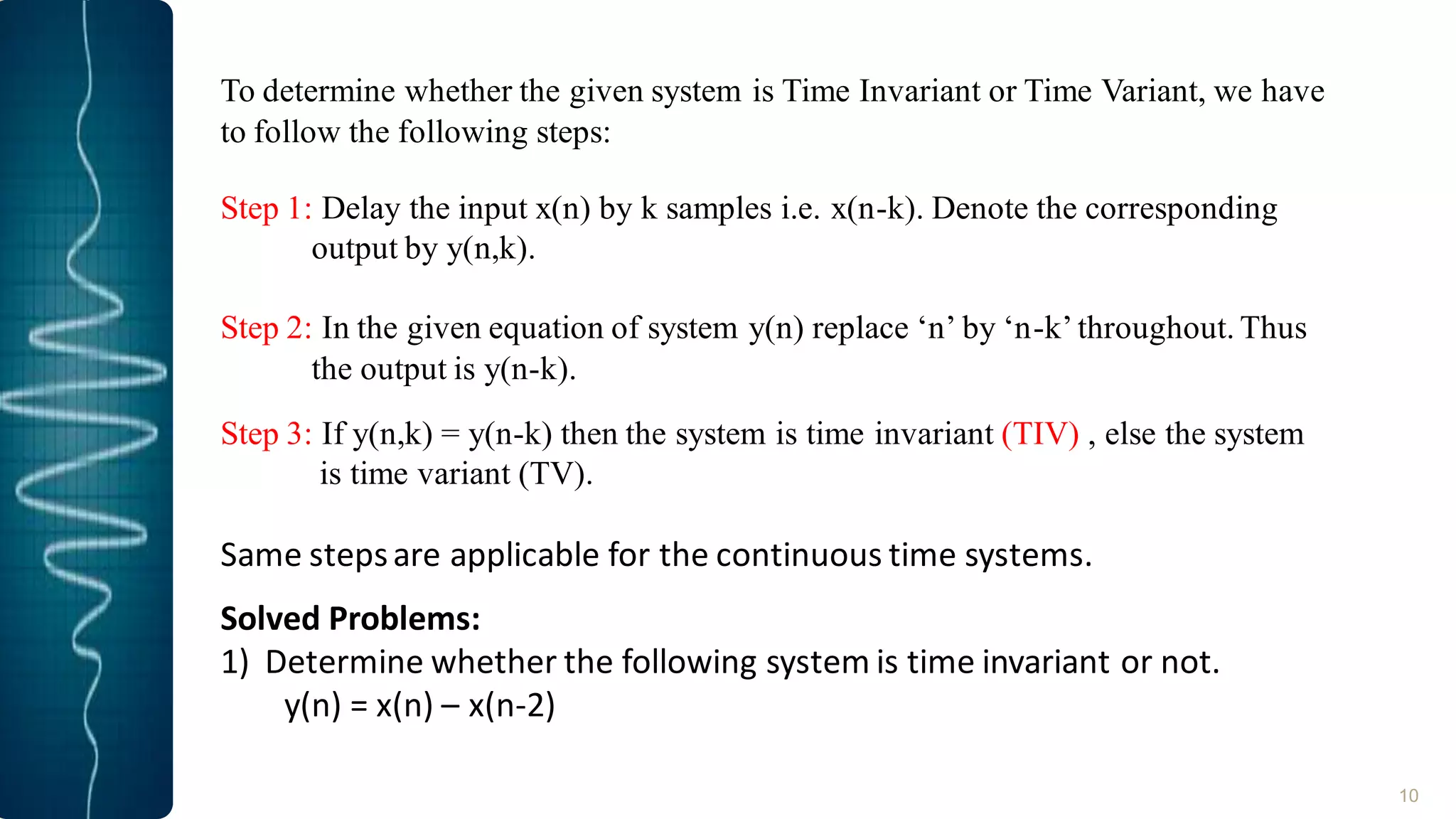
Theorem for linearity of the system:
A system is said to be linear if the combined response of a1x1(n) and a2x2(n) is equal to
the addition of the individual responses.
That means,
T[a1 x1(n) + a2 x2(n)] = a1 T[x1(n)] + a2 T[x2(n)]
The above theorem is also known as superposition theorem.
Important Characteristic:
Linear system has one important characteristic: If the input to the system is zero then it
produces zero output. If the given system produces some output (non-zero) at zero input
then the system is said to be Non-linear system. If this condition is satisfied then apply
the superposition theorem to determine whether the given system is linear or not?

14. 14
For continuous time system:
Similar to the discrete time system a continuous time system is said to be linear if it
follows the superposition theorem.
Let us consider two systems as follows:
y1(t) = f[x1(t)]
And y2(t) = f[x2(t)]
Here y1(t) and y2(t) are the responses of the system and x1(t) and x2(t) are the
excitations. Then the system is said to be linear if it satisfies the following expression:
f[a1 x1(t) + a2 x2(t)] = a1 y1(t) + a2 y2(t)
Where a1 and a2 are constants.
A system is said to be non-linear system if does not satisfies the above expression.

15. 15
Communication channels and filters are examples of linear systems.
How to determine whether the given system is Linear or not?
To determine whether the given system is Linear or not, we have to follow the following
steps:
Step 1: Apply zero input and check the output. If the output is zero then the system is
linear. If this step is satisfied then follow the remaining steps.
Step 2: Apply individual inputs to the system and determine corresponding outputs. Then
add all outputs. Denote this addition by y’(n).
Step 3: Combine all inputs. Apply it to the system and find out y”(n).
Step 4: if y’(n) = y”(n) then the system is linear otherwise it is non-linear system.

16. 16
Solved problem:
Determine whether the following system is linear or not?
y(n) = n x(n)
Solution:
Step 1: When input x(n) is zero then output is also zero. Here first step is satisfied so we
will check remaining steps for linearity.
Step 2: Let us consider two inputs x1(n) and x2(n) be the two inputs which produces
outputs y1(t) and y2(t) respectively. It is given as follows:

17. 17
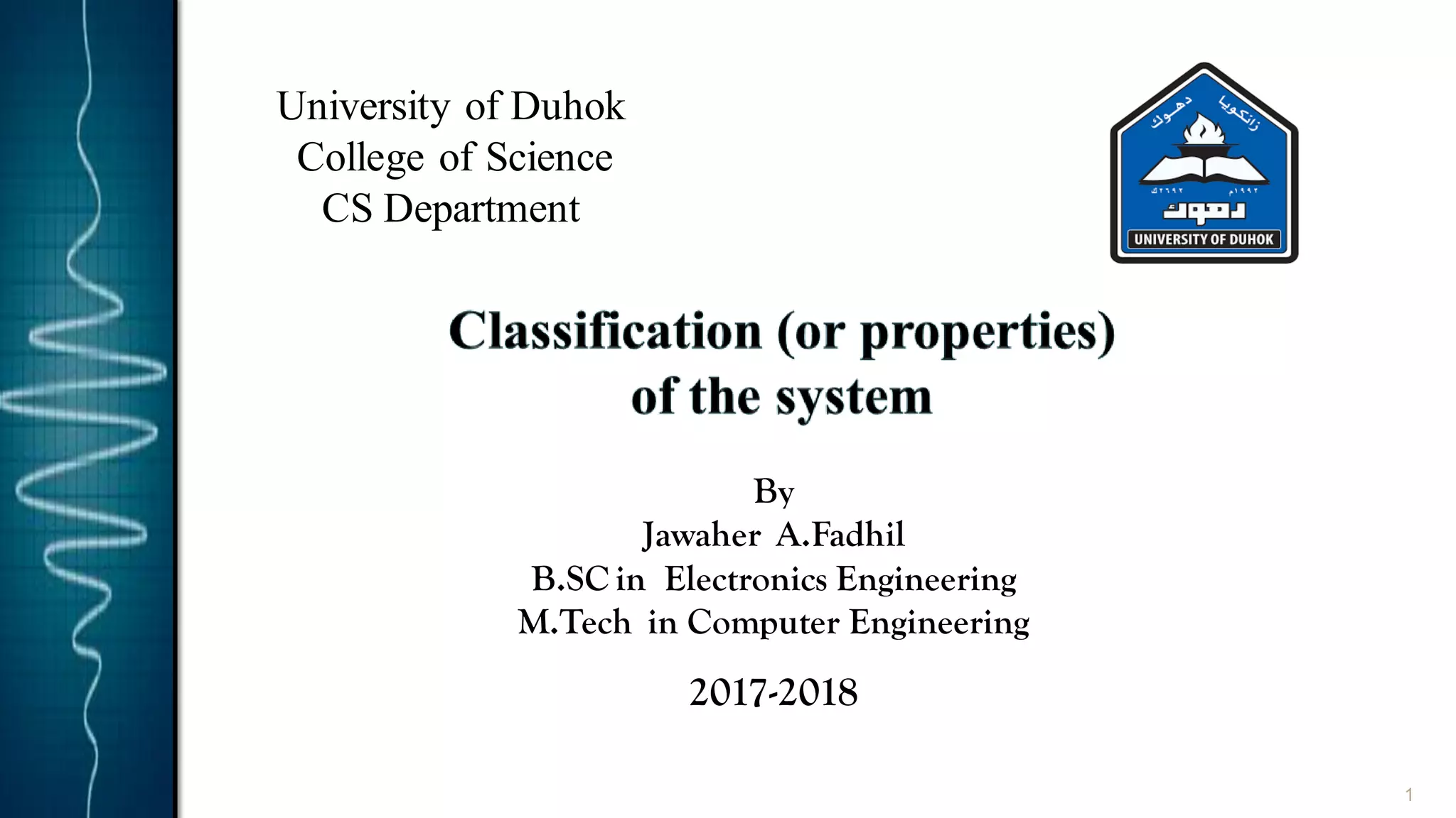
Now add these two output to get y’(n)
Therefore y’(n) = y1(n) + y2(n) = n x1(n) + n x2(n)
Therefore y’(n) = n [x1(n) + x2(n)]
Step 3: Now add x1(n) and x2(n) and apply this input to the system.
Therefore
We know that the function of system is to multiply input by ‘n’.
Here [x1(n) + x2(n)] acts as one input to the system. So the corresponding output is,
y”(n) = n [x1(n) + x2(n)]
Step 4: Compare y’(n) and y”(n).
Here y’(n) = y”(n). hence the given system is linear.

18. 18
Causal and Noncausal System (Causality Property)
A) Causal systems:
Definition: A system is said to be causal system if its output depends on present and past
inputs only and not on future inputs.
Examples: The output of casual system depends on present and past inputs, it means y(n) is a
function of x(n), x(n-1), x(n-2), x(n-3)…etc. Some examples of causal systems are given
below:
1) y(n) = x(n) + x(n-2)
2) y(n) = x(n-1) – x(n-3)
3) y(n) = 7x(n-5)
Significance of causal systems:
Since causal system does not include future input samples; such system is practically
realizable. That mean such system can be implemented practically. Generally all real time
systems are causal systems; because in real time applications only present and past samples
are present. Since future samples are not present; causal system is memory less system.

19. 19
B) Anti causal or non-causal system:
Definition: A system whose present response depends on future values of the inputs is
called as a non-causal system.
Examples: In this case, output y(n) is function of x(n), x(n-1), x(n-2)…etc. as well as it
is function of x(n+1), x(n+2), x(n+3), … etc. following are some examples of non-
causal systems:
1) Y(n) = x(n) + x(n+1)
2) Y(n) = 7x(n+2)
3) Y(n) = x(n) + 9x(n+5)
Significance of non-causal systems:
Since non-causal system contains future samples; a non-causal system is practically not
realizable. That means in practical cases it is not possible to implement a non-causal
system.

20. 20
But if the signals are stored in the memory and at a later time they are used by a system
then such signals are treated as advanced or future signal. Because such signals are
already present, before the system has started its operation. In such cases it is possible
to implement a non-causal system.
Some practical examples of non-causal systems are as follows:
1) Population growth
2) Weather forecasting
3) Planning commission etc.
For continuous time (C.T.) system:
A C.T. system is said to be “causal” if it produces a response y(t) only after the
application of excitation x(t). That means for a causal system the response does not
begin before the application of the input x(t).

21. 21
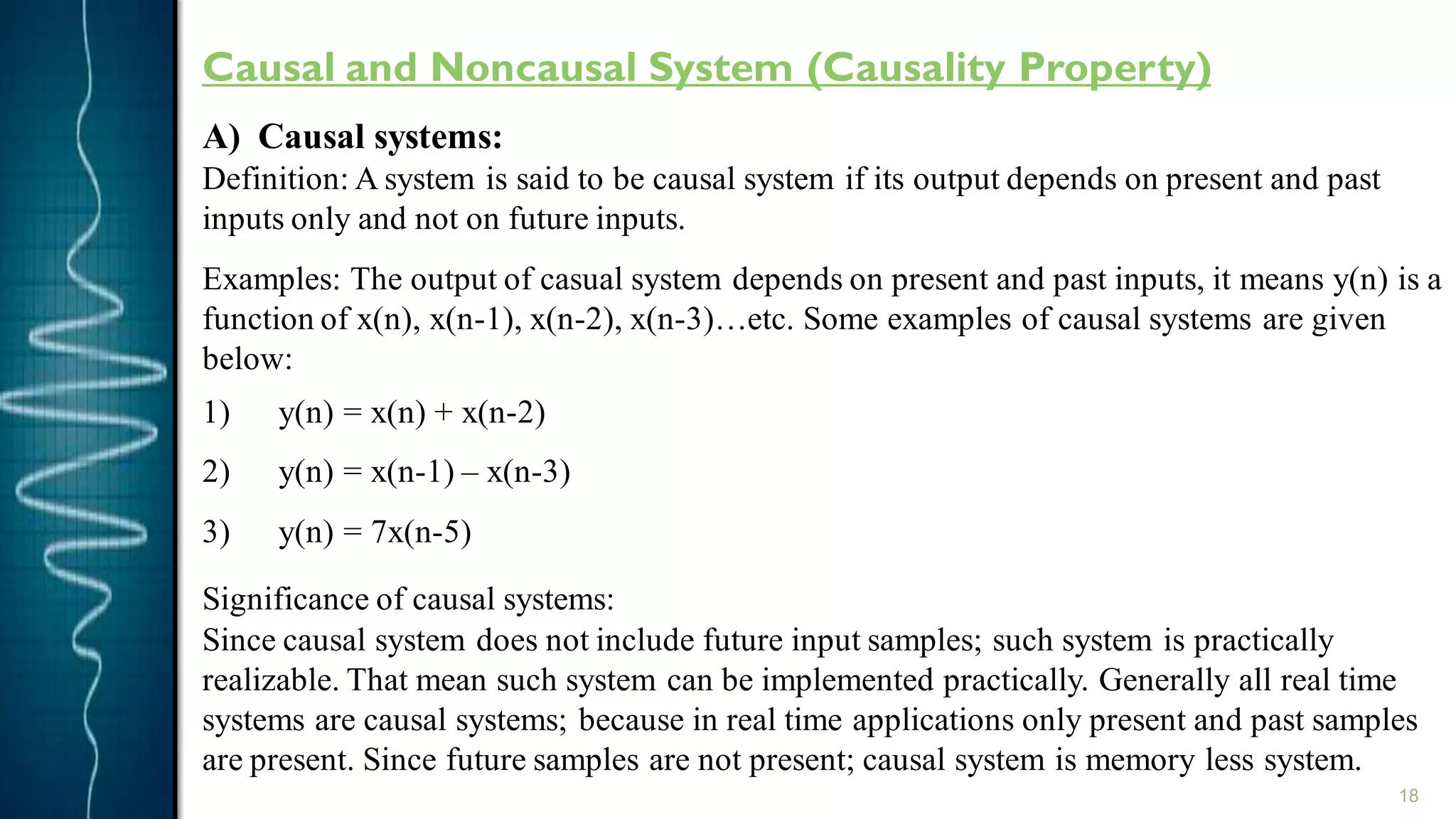
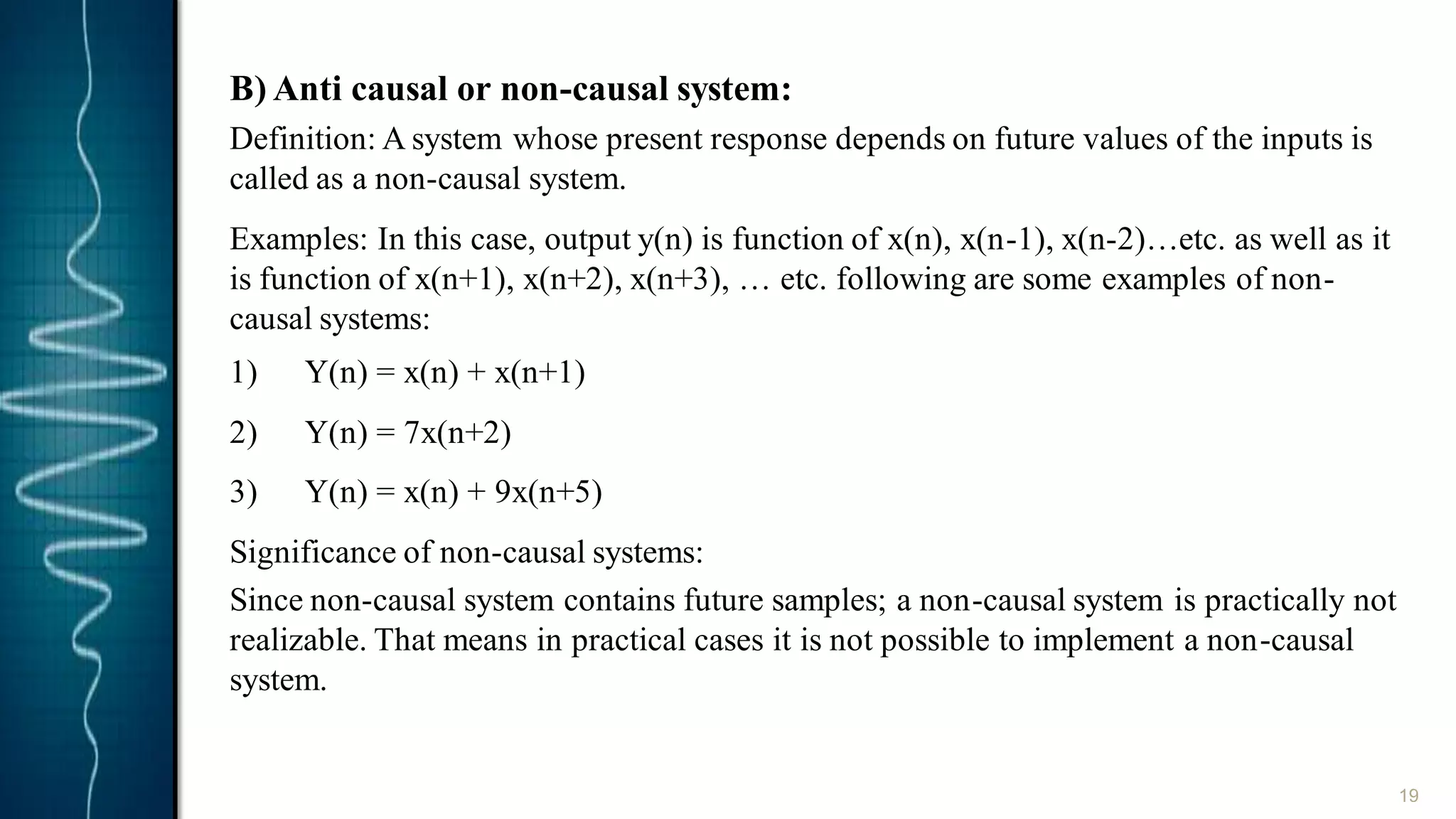
Solved problems on causal and non-causal system:
Determine if the systems described by the following equations are causal or non-causal.
1) y(n) = x(n) + x(n-3)
Solution: the given system is causal because its output (y(n)) depends only on the present
x(n) and past x(n-3) inputs.
2) y(n) = x(-n+2)
Solution:
this is non-causal system. This is because at n = -1 we get y(-1) = x[-(-1)+2] = x(3).
Thus present output at n = -1, expects future input i.e. x(3)

22. 22
Stable or Unstable System (Stability Property)
Definition of stable system:
An infinite system is BIBO stable if and only if every bounded input produces
bounded output.
Mathematical representation:
Let us consider some finite number Mx whose value is less than infinite. That
means Mx < , so it’s a finite value. Then if input is bounded, we can write,
|x(n)| = Mx <
Similarly for C.T. system
|x(t)| = Mx <
Similarly consider some finite number My whose value is less than infinity.
That means My < , so it’s a finite value. Then if output is bounded, we can
write,
|y(n)| = My <
Similarly for continuous time system
|y(t)| = My <
888
8
88

23. 23
Definition of Unstable system:
An initially system is said to be unstable if bounded input produces unbounded
(infinite) output.
Significance:
• Unstable system shows erratic and extreme behavior.
• When unstable system is practically implemented then it causes overflow.
Solved problem on stability:
Determine whether the following discrete time functions are stable or not.
• y(n) = x(-n)
Solution: we have to check the stability of the system by applying bounded
input. That means the value of x(-n) should be finite. So when input is bounded
output will be bounded. Thus the given function is Stable system.