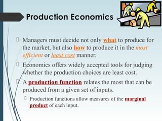
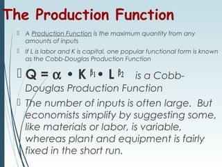
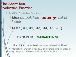
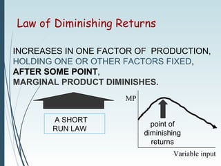
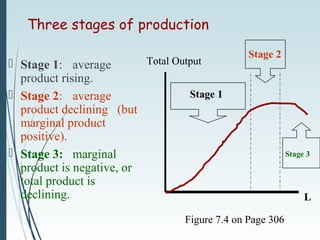
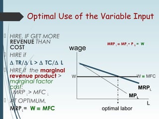
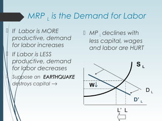
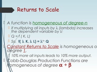
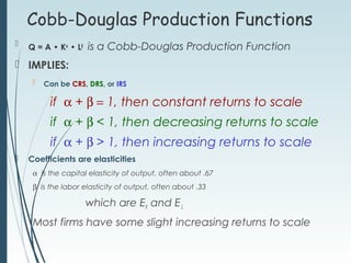
PRODUCTION
PREPARED BY –
VANSHIKA AGRAWAL
Production Economics
 Managers must decide not only what to produce for
the market, but also how to produce it in the most
efficient or least cost manner.
 Economics offers widely accepted tools for judging
whether the production choices are least cost.
 A production function relates the most that can be
produced from a given set of inputs.
 Production functions allow measures of the marginal
product of each input.
The Production Function
 A Production Function is the maximum quantity from any
amounts of inputs
 If L is labor and K is capital, one popular functional form is known
as the Cobb-Douglas Production Function
 Q = α • K β1• L β2 is a Cobb-
Douglas Production Function
 The number of inputs is often large. But
economists simplify by suggesting some,
like materials or labor, is variable,
whereas plant and equipment is fairly
fixed in the short run.
The Short Run
Production Function
 Short Run Production Functions:
 Max output, from a n y set of
inputs
 Q = f ( X1, X2, X3, X4, X5 ... )
FIXED IN SR VARIABLE IN SR
_
Q = f ( K, L) for two input case, where K as Fixed
 A Production Function is has only one variable input, labor, is
easily analyzed. The one variable input is labor, L.
 Average Product = Q / L
 output per labor
 Marginal Product = ∂ Q / ∂ L = dQ / dL
 output attributable to last unit of labor
applied
 Similar to profit functions, the Peak of MP
occurs before the Peak of average
product
 When MP = AP, we’re at the peak of
the AP curve
Elasticities of Production
 The production elasticity of labor,
 EL = MPL / APL = (∆Q/∆L) / (Q/L) = (∆Q/∆L)·(L/Q)
 The production elasticity of capital has the identical in form, except K appears in place
of L.
 When MPL > APL, then the labor elasticity, EL > 1.
 A 1 percent increase in labor will increase output by
more than 1 percent.
 When MPL < APL, then the labor elasticity, EL < 1.
 A 1 percent increase in labor will increase output by less
than 1 percent.
Short Run Production Function
Numerical Example
L Q MP AP
0 0 --- ---
1 20 20 20
2 46 26 23
3
4
5
70
92
110
24
22
18
23.33
23
22
Marginal Product
L
1 2 3 4 5
Average
Product
Labor Elasticity is greater then one,
for labor use up through L = 3 units
 When MP > AP, then AP is RISING
 IF YOUR MARGINAL GRADE IN THIS CLASS IS
HIGHER THAN YOUR GRADE POINT AVERAGE,
THEN YOUR G.P.A. IS RISING
 When MP < AP, then AP is FALLING
 IF YOUR MARGINAL BATTING AVERAGE IS LESS
THAN THAT OF THE NEW YORK YANKEES, YOUR
ADDITION TO THE TEAM WOULD LOWER THE
YANKEE’S TEAM BATTING AVERAGE
 When MP = AP, then AP is at its MAX
 IF THE NEW HIRE IS JUST AS EFFICIENT AS THE
AVERAGE EMPLOYEE, THEN AVERAGE
PRODUCTIVITY DOESN’T CHANGE
Law of Diminishing Returns
INCREASES IN ONE FACTOR OF PRODUCTION,
HOLDING ONE OR OTHER FACTORS FIXED,
AFTER SOME POINT,
MARGINAL PRODUCT DIMINISHES.
A SHORT
RUN LAW
point of
diminishing
returns
Variable input
MP
Figure 7.4 on Page 306
Three stages of production
 Stage 1: average
product rising.
 Stage 2: average
product declining (but
marginal product
positive).
 Stage 3: marginal
product is negative, or
total product is
declining. L
Total Output
Stage 1
Stage 2
Stage 3
Optimal Use of the Variable Input
 HIRE, IF GET MORE
REVENUE THAN
COST
 HIRE if
∆ TR/∆ L > ∆ TC/∆ L
 HIRE if the marginal
revenue product >
marginal factor
cost:
MRP L > MFC L
 AT OPTIMUM,
MRPL = W ≡ MFC
MRP L ≡ MPL • P Q = W
optimal labor
MPL
MRPL
W W ≡ MFC
L
wage
•
MRP L is the Demand for Labor
 If Labor is MORE
productive, demand
for labor increases
 If Labor is LESS
productive, demand
for labor decreases
 Suppose an EARTHQUAKEEARTHQUAKE
destroys capital →
 MP L declines with
less capital, wages
and labor are HURT
D L
D’ L
S L
W↓
L’ L
Long Run Production Functions
 All inputs are variable
 greatest output from any set of inputs
 Q = f( K, L ) is two input example
 MP of capital and MP of labor are the
derivatives of the production function
 MPL = ∂ Q / ∂ L = ∆Q / ∆L
 MP of labor declines as more labor is
applied. Also the MP of capital declines
as more capital is applied.
Isoquants & LR Production Functions
 In the LONG RUN, ALL
factors are variable
 Q = f ( K, L )
 ISOQUANTS -- locus of
input combinations
which produces the
same output (A & B or
on the same isoquant)
 SLOPE of ISOQUANT is
ratio of Marginal
Products, called the
MRTS, the marginal rate
of technical substitution
ISOQUANT MAP
B
A
C
Q1
Q2
Q3
K
L
Optimal Combination of Inputs
 The objective is to
minimize cost for a given
output
 ISOCOST lines are the
combination of inputs for a
given cost, C0
 C0 = CL·L + CK·K
 K = C0/CK - (CL/CK)·L
 Optimal where:
 MPL/MPK = CL/CK·
 Rearranged, this becomes the
equimarginal criterion
Equimarginal Criterion: Produce
where MPL/CL =
MPK/CK where marginal
products per dollar are
equal
Figure 7.9 on page 316
Q(1)
D
L
K
at D, slope of
isocost = slope
of isoquant
C(1)
Use of the Equimarginal Criterion
 Q: Is the following firm
EFFICIENT?
 Suppose that:
 MPL = 30
 MPK = 50
 W = 10 (cost of labor)
 R = 25 (cost of capital)
 Labor: 30/10 = 3
 Capital: 50/25 = 2
 A: No!
 A dollar spent on labor
produces 3, and a dollar
spent on capital produces 2.
USE RELATIVELY MORE
LABOR!
 If spend $1 less in capital,
output falls 2 units, but rises 3
units when spent on labor
 Shift to more labor until the
equimarginal condition
holds.
 That is peak efficiency.
Allocative & Technical Efficiency
 Allocative Efficiency – asks if the firm using the least cost combination of
input
 It satisfies: MPL/CL = MPK/CK
 Technical Efficiency – asks if the firm is maximizing potential output from a
given set of inputs
 When a firm produces at point T rather
than point D on a lower
isoquant, they firm is not
producing as much as is
technically possible.
Q(1)
D
Q(0)
T
Returns to Scale
 A function is homogeneous of degree-n
 if multiplying all inputs by λ (lambda) increases
the dependent variable by λn
 Q = f ( K, L)
 So, f( λ K, λ L) = λn•
Q
 Constant Returns to Scale is homogeneous o
degree 1.
 10% more all inputs leads to 10% more output.
 Cobb-Douglas Production Functions are
homogeneous of degree α + β
Cobb-Douglas Production Functions
 Q = A • Kα
• Lβ
is a Cobb-Douglas Production Function
 IMPLIES:
 Can be CRS, DRS, or IRS
if α + β = 1, then constant returns to scale
if α + β < 1, then decreasing returns to scale
if α + β > 1, then increasing returns to scale
 Coefficients are elasticities
α is the capital elasticity of output, often about .67
β is the labor elasticity of output, often about .33
which are EK and EL
Most firms have some slight increasing returns to scale
PRODUCTION CONCEPT

PRODUCTION CONCEPT

  • 1.
  • 2.
    Production Economics  Managersmust decide not only what to produce for the market, but also how to produce it in the most efficient or least cost manner.  Economics offers widely accepted tools for judging whether the production choices are least cost.  A production function relates the most that can be produced from a given set of inputs.  Production functions allow measures of the marginal product of each input.
  • 3.
    The Production Function A Production Function is the maximum quantity from any amounts of inputs  If L is labor and K is capital, one popular functional form is known as the Cobb-Douglas Production Function  Q = α • K β1• L β2 is a Cobb- Douglas Production Function  The number of inputs is often large. But economists simplify by suggesting some, like materials or labor, is variable, whereas plant and equipment is fairly fixed in the short run.
  • 4.
    The Short Run ProductionFunction  Short Run Production Functions:  Max output, from a n y set of inputs  Q = f ( X1, X2, X3, X4, X5 ... ) FIXED IN SR VARIABLE IN SR _ Q = f ( K, L) for two input case, where K as Fixed  A Production Function is has only one variable input, labor, is easily analyzed. The one variable input is labor, L.
  • 5.
     Average Product= Q / L  output per labor  Marginal Product = ∂ Q / ∂ L = dQ / dL  output attributable to last unit of labor applied  Similar to profit functions, the Peak of MP occurs before the Peak of average product  When MP = AP, we’re at the peak of the AP curve
  • 6.
    Elasticities of Production The production elasticity of labor,  EL = MPL / APL = (∆Q/∆L) / (Q/L) = (∆Q/∆L)·(L/Q)  The production elasticity of capital has the identical in form, except K appears in place of L.  When MPL > APL, then the labor elasticity, EL > 1.  A 1 percent increase in labor will increase output by more than 1 percent.  When MPL < APL, then the labor elasticity, EL < 1.  A 1 percent increase in labor will increase output by less than 1 percent.
  • 7.
    Short Run ProductionFunction Numerical Example L Q MP AP 0 0 --- --- 1 20 20 20 2 46 26 23 3 4 5 70 92 110 24 22 18 23.33 23 22 Marginal Product L 1 2 3 4 5 Average Product Labor Elasticity is greater then one, for labor use up through L = 3 units
  • 8.
     When MP> AP, then AP is RISING  IF YOUR MARGINAL GRADE IN THIS CLASS IS HIGHER THAN YOUR GRADE POINT AVERAGE, THEN YOUR G.P.A. IS RISING  When MP < AP, then AP is FALLING  IF YOUR MARGINAL BATTING AVERAGE IS LESS THAN THAT OF THE NEW YORK YANKEES, YOUR ADDITION TO THE TEAM WOULD LOWER THE YANKEE’S TEAM BATTING AVERAGE  When MP = AP, then AP is at its MAX  IF THE NEW HIRE IS JUST AS EFFICIENT AS THE AVERAGE EMPLOYEE, THEN AVERAGE PRODUCTIVITY DOESN’T CHANGE
  • 9.
    Law of DiminishingReturns INCREASES IN ONE FACTOR OF PRODUCTION, HOLDING ONE OR OTHER FACTORS FIXED, AFTER SOME POINT, MARGINAL PRODUCT DIMINISHES. A SHORT RUN LAW point of diminishing returns Variable input MP
  • 10.
    Figure 7.4 onPage 306 Three stages of production  Stage 1: average product rising.  Stage 2: average product declining (but marginal product positive).  Stage 3: marginal product is negative, or total product is declining. L Total Output Stage 1 Stage 2 Stage 3
  • 11.
    Optimal Use ofthe Variable Input  HIRE, IF GET MORE REVENUE THAN COST  HIRE if ∆ TR/∆ L > ∆ TC/∆ L  HIRE if the marginal revenue product > marginal factor cost: MRP L > MFC L  AT OPTIMUM, MRPL = W ≡ MFC MRP L ≡ MPL • P Q = W optimal labor MPL MRPL W W ≡ MFC L wage •
  • 12.
    MRP L isthe Demand for Labor  If Labor is MORE productive, demand for labor increases  If Labor is LESS productive, demand for labor decreases  Suppose an EARTHQUAKEEARTHQUAKE destroys capital →  MP L declines with less capital, wages and labor are HURT D L D’ L S L W↓ L’ L
  • 13.
    Long Run ProductionFunctions  All inputs are variable  greatest output from any set of inputs  Q = f( K, L ) is two input example  MP of capital and MP of labor are the derivatives of the production function  MPL = ∂ Q / ∂ L = ∆Q / ∆L  MP of labor declines as more labor is applied. Also the MP of capital declines as more capital is applied.
  • 14.
    Isoquants & LRProduction Functions  In the LONG RUN, ALL factors are variable  Q = f ( K, L )  ISOQUANTS -- locus of input combinations which produces the same output (A & B or on the same isoquant)  SLOPE of ISOQUANT is ratio of Marginal Products, called the MRTS, the marginal rate of technical substitution ISOQUANT MAP B A C Q1 Q2 Q3 K L
  • 15.
    Optimal Combination ofInputs  The objective is to minimize cost for a given output  ISOCOST lines are the combination of inputs for a given cost, C0  C0 = CL·L + CK·K  K = C0/CK - (CL/CK)·L  Optimal where:  MPL/MPK = CL/CK·  Rearranged, this becomes the equimarginal criterion Equimarginal Criterion: Produce where MPL/CL = MPK/CK where marginal products per dollar are equal Figure 7.9 on page 316 Q(1) D L K at D, slope of isocost = slope of isoquant C(1)
  • 16.
    Use of theEquimarginal Criterion  Q: Is the following firm EFFICIENT?  Suppose that:  MPL = 30  MPK = 50  W = 10 (cost of labor)  R = 25 (cost of capital)  Labor: 30/10 = 3  Capital: 50/25 = 2  A: No!  A dollar spent on labor produces 3, and a dollar spent on capital produces 2. USE RELATIVELY MORE LABOR!  If spend $1 less in capital, output falls 2 units, but rises 3 units when spent on labor  Shift to more labor until the equimarginal condition holds.  That is peak efficiency.
  • 17.
    Allocative & TechnicalEfficiency  Allocative Efficiency – asks if the firm using the least cost combination of input  It satisfies: MPL/CL = MPK/CK  Technical Efficiency – asks if the firm is maximizing potential output from a given set of inputs  When a firm produces at point T rather than point D on a lower isoquant, they firm is not producing as much as is technically possible. Q(1) D Q(0) T
  • 18.
    Returns to Scale A function is homogeneous of degree-n  if multiplying all inputs by λ (lambda) increases the dependent variable by λn  Q = f ( K, L)  So, f( λ K, λ L) = λn• Q  Constant Returns to Scale is homogeneous o degree 1.  10% more all inputs leads to 10% more output.  Cobb-Douglas Production Functions are homogeneous of degree α + β
  • 19.
    Cobb-Douglas Production Functions Q = A • Kα • Lβ is a Cobb-Douglas Production Function  IMPLIES:  Can be CRS, DRS, or IRS if α + β = 1, then constant returns to scale if α + β < 1, then decreasing returns to scale if α + β > 1, then increasing returns to scale  Coefficients are elasticities α is the capital elasticity of output, often about .67 β is the labor elasticity of output, often about .33 which are EK and EL Most firms have some slight increasing returns to scale