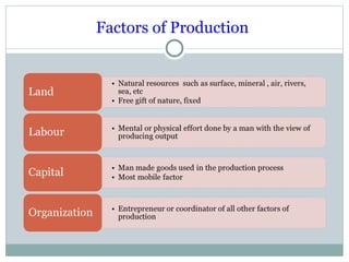
Theory of Production
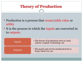
Production is a process that create/adds value or
utility
It is the process in which the inputs are converted in
to outputs.
3.
Production Function
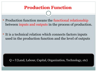
Productionfunction means the functional relationship
between inputs and outputs in the process of production.
It is a technical relation which connects factors inputs
used in the production function and the level of outputs
Q = f (Land, Labour, Capital, Organization, Technology, etc)
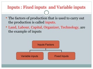
Inputs : Fixedinputs and Variable inputs
The factors of production that is used to carry out
the production is called inputs.
Land, Labour, Capital, Organizer, Technology, are
the example of inputs
Inputs Factors
Variable inputs Fixed Inputs
6.
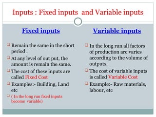
Inputs : Fixedinputs and Variable inputs
Fixed inputs
Remain the same in the short
period .
At any level of out put, the
amount is remain the same.
The cost of these inputs are
called Fixed Cost
Examples:- Building, Land
etc
( In the long run fixed inputs
become variable)
Variable inputs
In the long run all factors
of production are varies
according to the volume of
outputs.
The cost of variable inputs
is called Variable Cost
Example:- Raw materials,
labour, etc
7.
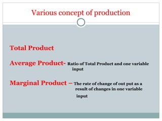
Total Product
Average Product-Ratio of Total Product and one variable
input
Marginal Product – The rate of change of out put as a
result of changes in one variable
input
Various concept of production
8.
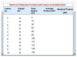
Production with OneVariable Input
Labour
(L)
Capital
(K)
Total
Output
(TP)
Average
Product (AP)
0
1
2
3
4
5
6
7
8
9
10
10
10
10
10
10
10
10
10
10
10
10
Marginal Product
(MP)
0
10
30
60
80
95
108
112
112
108
100
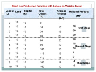
Short run Production Function with Labour as Variable factor
9.
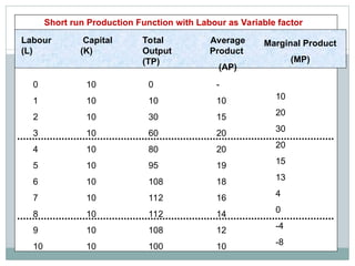
Production with OneVariable Input
Labour
(L)
Capital
(K)
Total
Output
(TP)
Average
Product
(AP)
0
1
2
3
4
5
6
7
8
9
10
10
10
10
10
10
10
10
10
10
10
10
0
10
30
60
80
95
108
112
112
108
100
10
20
30
20
15
13
4
0
-4
-8
-
10
15
20
20
19
18
16
14
12
10
Marginal Product
(MP)
Short run Production Function with Labour as Variable factor
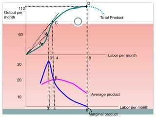
10.
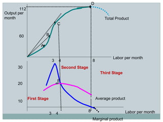
A
C
B
Total Product
Labor permonth
3
4 8
8
4
3
E
Average product
Marginal product
Output per
month
112
Labor per month
60
30
20
10
D
11.
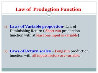
Law of ProductionFunction
1) Laws of Variable proportion- Law of
Diminishing Return ( Short run production
function with at least one input is variable)
2) Laws of Return scales – Long run production
function with all inputs factors are variable.
12.
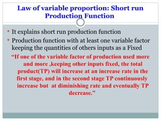
Law of variableproportion: Short run
Production Function
It explains short run production function
Production function with at least one variable factor
keeping the quantities of others inputs as a Fixed
“If one of the variable factor of production used more
and more ,keeping other inputs fixed, the total
product(TP) will increase at an increase rate in the
first stage, and in the second stage TP continuously
increase but at diminishing rate and eventually TP
decrease.”
13.
Production with OneVariable Input
Labour
(L)
Capital
(K)
Total
Output
(TP)
Average
Product
(AP)
0
1
2
3
4
5
6
7
8
9
10
10
10
10
10
10
10
10
10
10
10
10
0
10
30
60
80
95
108
112
112
108
100
10
20
30
20
15
13
4
0
-4
-8
-
10
15
20
20
19
18
16
14
12
10
Marginal Product
(MP)
10
10
10
10
10
10
10
10
10
10
10
Land
First Stage
Second Stage
Third Stage
Short run Production Function with Labour as Variable factor
14.
A
C
B
Total Product
Labor permonth
3
4 8
8
4
3
E
Average product
Marginal product
Output per
month
112
Labor per month
60
30
20
10
D
First Stage
Second Stage
Third Stage
15.
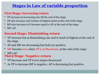
Stages in Lawof variable proportion
First Stage: Increasing return
TP increase at increasing rate till the end of the stage.
AP also increase and reaches at highest point at the end of the stage.
MP also increase at it become equal to AP at the end of the stage.
MP>AP
Second Stage: Diminishing return
TP increase but at diminishing rate and it reach at highest at the end of
the stage.
AP and MP are decreasing but both are positive.
MP become zero when TP is at Maximum, at the end of the stage
MP<AP.
Third Stage: Negative return
TP decrease and TP Curve slopes downward
As TP is decrease MP is negative. AP is decreasing but positive.
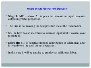
Stage I:MP is above AP implies an increase in input increases
output in greater proportion.
The firm is not making the best possible use of the fixed factor.
So, the firm has an incentive to increase input until it crosses over
to stage II.
Stage III: MP is negative implies contribution of additional labor
is negative so the total output decreases .
In this case it will be unwise to employ an additional labor.
Where should rational firm produce?
18.
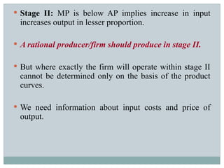
Stage II:MP is below AP implies increase in input
increases output in lesser proportion.
A rational producer/firm should produce in stage II.
But where exactly the firm will operate within stage II
cannot be determined only on the basis of the product
curves.
We need information about input costs and price of
output.
19.
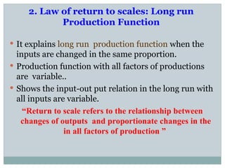
2. Law ofreturn to scales: Long run
Production Function
It explains long run production function when the
inputs are changed in the same proportion.
Production function with all factors of productions
are variable..
Shows the input-out put relation in the long run with
all inputs are variable.
“Return to scale refers to the relationship between
changes of outputs and proportionate changes in the
in all factors of production ”
20.
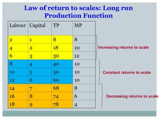
Law of returnto scales: Long run
Production Function
Labour Capital TP MP
2 1 8 8
4 2 18 10
6 3 30 12
8 4 40 10
10 5 50 10
12 6 60 10
14 7 68 8
16 8 74 6
18 9 78 4
Increasing returns to scale
Constant returns to scale
Decreasing returns to scale
21.
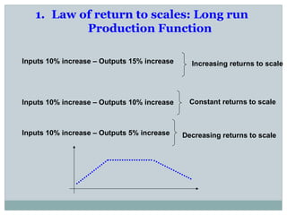
1. Law ofreturn to scales: Long run
Production Function
Increasing returns to scale
Constant returns to scale
Decreasing returns to scale
Inputs 10% increase – Outputs 15% increase
Inputs 10% increase – Outputs 10% increase
Inputs 10% increase – Outputs 5% increase
22.
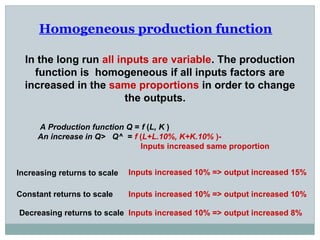
Homogeneous production function
Inthe long run all inputs are variable. The production
function is homogeneous if all inputs factors are
increased in the same proportions in order to change
the outputs.
A Production function Q = f (L, K )
An increase in Q> Q^ = f (L+L.10%, K+K.10% )-
Inputs increased same proportion
Increasing returns to scale
Constant returns to scale
Decreasing returns to scale
Inputs increased 10% => output increased 15%
Inputs increased 10% => output increased 10%
Inputs increased 10% => output increased 8%
23.
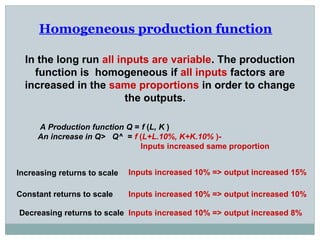
Homogeneous production function
Inthe long run all inputs are variable. The production
function is homogeneous if all inputs factors are
increased in the same proportions in order to change
the outputs.
A Production function Q = f (L, K )
An increase in Q> Q^ = f (L+L.10%, K+K.10% )-
Inputs increased same proportion
Increasing returns to scale
Constant returns to scale
Decreasing returns to scale
Inputs increased 10% => output increased 15%
Inputs increased 10% => output increased 10%
Inputs increased 10% => output increased 8%
24.
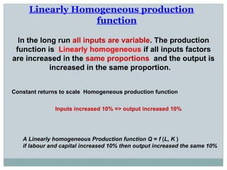
Linearly Homogeneous production
function
Inthe long run all inputs are variable. The production
function is Linearly homogeneous if all inputs factors
are increased in the same proportions and the output is
increased in the same proportion.
Constant returns to scale Homogeneous production function
Inputs increased 10% => output increased 10%
A Linearly homogeneous Production function Q = f (L, K )
if labour and capital increased 10% then output increased the same 10%
25.
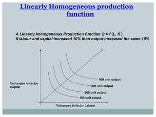
Linearly Homogeneous production
function
ALinearly homogeneous Production function Q = f (L, K )
if labour and capital increased 10% then output increased the same 10%
100 unit output
200 unit output
300 unit output
400 unit output
%changes in factor Labour
%changes in factor
Capital
26.
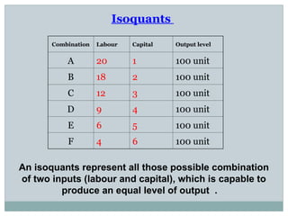
Isoquants
Combination Labour CapitalOutput level
A 20 1 100 unit
B 18 2 100 unit
C 12 3 100 unit
D 9 4 100 unit
E 6 5 100 unit
F 4 6 100 unit
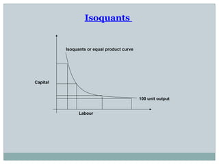
An isoquants represent all those possible combination
of two inputs (labour and capital), which is capable to
produce an equal level of output .
100 unit output
Labour
Capital
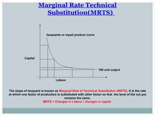
Isoquantsor equal product curve
Marginal Rate Technical
Substitution(MRTS)
The slope of isoquant is known as Marginal Rate of Technical Substitution (MRTS). It is the rate
at which one factor of production is substituted with other factor so that the level of the out put
remains the same.
MRTS = Changes in Labour / changes in capital