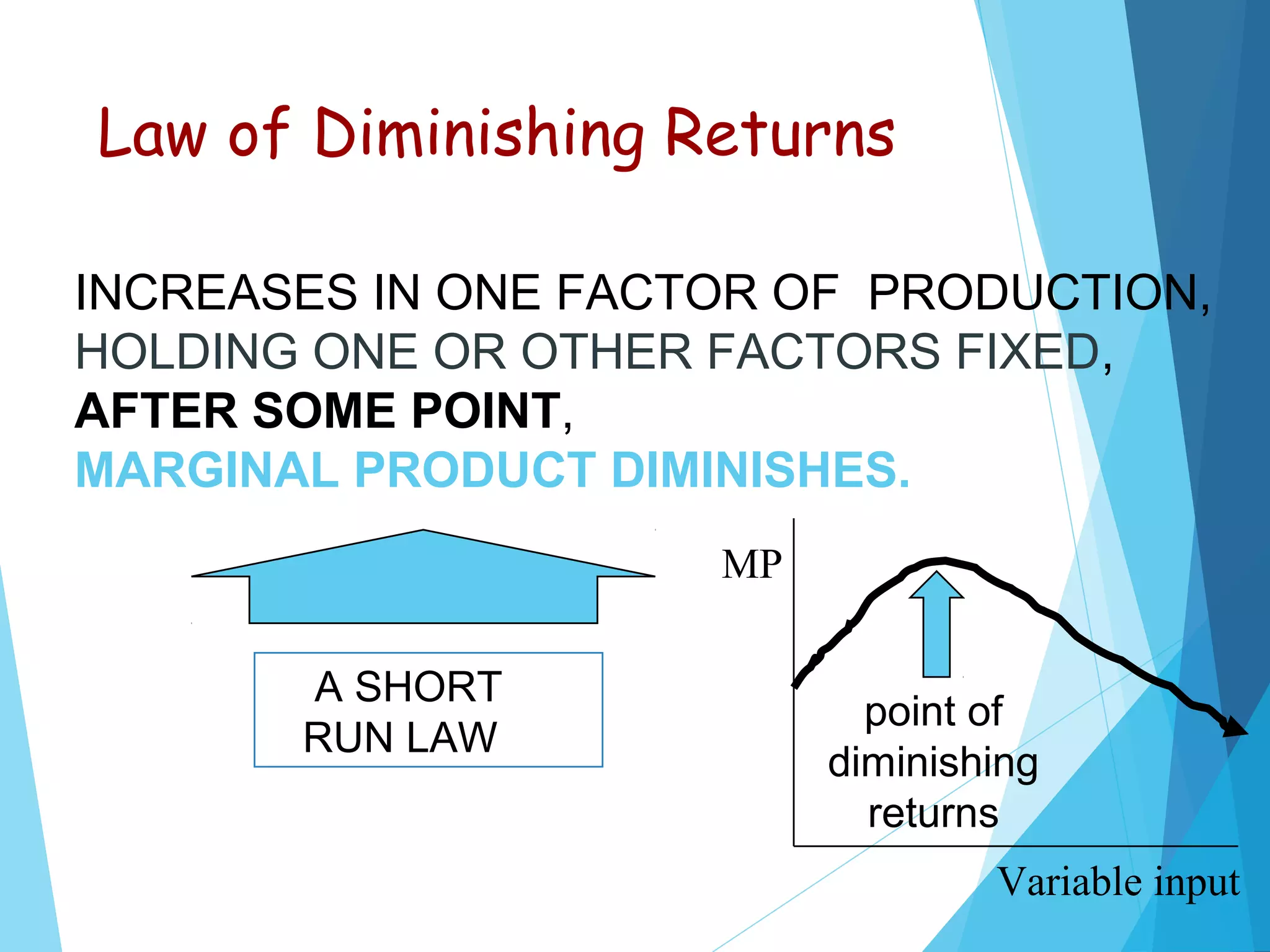
©2005 South-Western Publishing
Production Economics
 Managers must decide not only what to produce for
the market, but also how to produce it in the most
efficient or least cost manner.
 Economics offers widely accepted tools for judging
whether the production choices are least cost.
 A production function relates the most that can be
produced from a given set of inputs.
The Production Function
 A Production Function is the maximum quantity from any amounts of inputs
 If L is labor and K is capital, one popular functional form is known as the Cobb-
Douglas Production Function.
 The number of inputs is often large. But economists
simplify by suggesting some, like materials or labor,
is variable, whereas plant and equipment is fairly
fixed in the short run.
Average Product
output per labor
Marginal Product
output attributable to last unit of labor
applied.
Similar to profit functions, the Peak of
MP occurs before the Peak of average
product.
Short Run Production Function
Numerical Example
L Q MP AP
0 0 --- ---
1 20 20 20
2 46 26 23
3
4
5
70
92
110
24
22
18
23.33
23
22
Marginal Product
L
1 2 3 4 5
Average
Product
Labor Elasticity is greater then one,
for labor use up through L = 3 units
When MP > AP, then AP is RISING
 IF YOUR MARGINAL GRADE IN THIS CLASS IS HIGHER
THAN YOUR GRADE POINT AVERAGE, THEN YOUR
G.P.A. IS RISING
When MP < AP, then AP is FALLING
 IF YOUR MARGINAL BATTING AVERAGE IS LESS THAN
THAT OF THE NEW YORK YANKEES, YOUR ADDITION
TO THE TEAM WOULD LOWER THE YANKEE’S TEAM
BATTING AVERAGE
When MP = AP, then AP is at its MAX
 IF THE NEW HIRE IS JUST AS EFFICIENT AS THE
AVERAGE EMPLOYEE, THEN AVERAGE PRODUCTIVITY
DOESN’T CHANGE
Law of Diminishing Returns
INCREASES IN ONE FACTOR OF PRODUCTION,
HOLDING ONE OR OTHER FACTORS FIXED,
AFTER SOME POINT,
MARGINAL PRODUCT DIMINISHES.
A SHORT
RUN LAW
point of
diminishing
returns
Variable input
MP
Figure 7.4 on Page 306
Three stages of production
 Stage 1: average
product rising.
 Stage 2: average
product declining (but
marginal product
positive).
 Stage 3: marginal
product is negative, or
total product is
declining. L
Total Output
Stage 1
Stage 2
Stage 3
Isoquants & LR Production Functions
 In the LONG RUN, ALL
factors are variable
 Q = f ( K, L )
 ISOQUANTS -- locus of
input combinations which
produces the same output
(A & B or on the same
isoquant)
 SLOPE of ISOQUANT is
ratio of Marginal
Products, called the
MRTS, the marginal rate
of technical substitution
ISOQUANT MAP
B
A
C
Q1
Q2
Q3
K
L
Cobb-Douglas Production Functions

Q = A • Kα
• Lβ
is a Cobb-Douglas Production Function
 IMPLIES:
 Can be CRS, DRS, or IRS
if α + β = 1, then constant returns to scale
if α + β < 1, then decreasing returns to scale
if α + β > 1, then increasing returns to scale
 Coefficients are elasticities
α is the capital elasticity of output, often about .67
β is the labor elasticity of output, often about .33
which are EK and EL
Most firms have some slight increasing returns to scale

PRODUCTION CONCEPT

  • 2.
    ©2005 South-Western Publishing ProductionEconomics  Managers must decide not only what to produce for the market, but also how to produce it in the most efficient or least cost manner.  Economics offers widely accepted tools for judging whether the production choices are least cost.  A production function relates the most that can be produced from a given set of inputs.
  • 3.
    The Production Function A Production Function is the maximum quantity from any amounts of inputs  If L is labor and K is capital, one popular functional form is known as the Cobb- Douglas Production Function.  The number of inputs is often large. But economists simplify by suggesting some, like materials or labor, is variable, whereas plant and equipment is fairly fixed in the short run.
  • 4.
    Average Product output perlabor Marginal Product output attributable to last unit of labor applied. Similar to profit functions, the Peak of MP occurs before the Peak of average product.
  • 5.
    Short Run ProductionFunction Numerical Example L Q MP AP 0 0 --- --- 1 20 20 20 2 46 26 23 3 4 5 70 92 110 24 22 18 23.33 23 22 Marginal Product L 1 2 3 4 5 Average Product Labor Elasticity is greater then one, for labor use up through L = 3 units
  • 6.
    When MP >AP, then AP is RISING  IF YOUR MARGINAL GRADE IN THIS CLASS IS HIGHER THAN YOUR GRADE POINT AVERAGE, THEN YOUR G.P.A. IS RISING When MP < AP, then AP is FALLING  IF YOUR MARGINAL BATTING AVERAGE IS LESS THAN THAT OF THE NEW YORK YANKEES, YOUR ADDITION TO THE TEAM WOULD LOWER THE YANKEE’S TEAM BATTING AVERAGE When MP = AP, then AP is at its MAX  IF THE NEW HIRE IS JUST AS EFFICIENT AS THE AVERAGE EMPLOYEE, THEN AVERAGE PRODUCTIVITY DOESN’T CHANGE
  • 7.
    Law of DiminishingReturns INCREASES IN ONE FACTOR OF PRODUCTION, HOLDING ONE OR OTHER FACTORS FIXED, AFTER SOME POINT, MARGINAL PRODUCT DIMINISHES. A SHORT RUN LAW point of diminishing returns Variable input MP
  • 8.
    Figure 7.4 onPage 306 Three stages of production  Stage 1: average product rising.  Stage 2: average product declining (but marginal product positive).  Stage 3: marginal product is negative, or total product is declining. L Total Output Stage 1 Stage 2 Stage 3
  • 9.
    Isoquants & LRProduction Functions  In the LONG RUN, ALL factors are variable  Q = f ( K, L )  ISOQUANTS -- locus of input combinations which produces the same output (A & B or on the same isoquant)  SLOPE of ISOQUANT is ratio of Marginal Products, called the MRTS, the marginal rate of technical substitution ISOQUANT MAP B A C Q1 Q2 Q3 K L
  • 10.
    Cobb-Douglas Production Functions  Q= A • Kα • Lβ is a Cobb-Douglas Production Function  IMPLIES:  Can be CRS, DRS, or IRS if α + β = 1, then constant returns to scale if α + β < 1, then decreasing returns to scale if α + β > 1, then increasing returns to scale  Coefficients are elasticities α is the capital elasticity of output, often about .67 β is the labor elasticity of output, often about .33 which are EK and EL Most firms have some slight increasing returns to scale