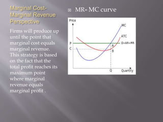
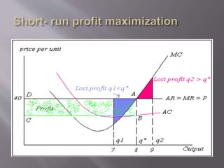
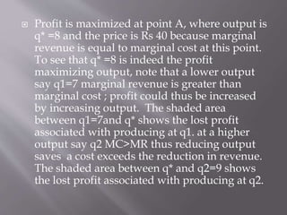
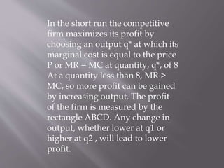
1) A firm produces at the quantity where marginal revenue equals marginal cost to maximize profits. This is the point where additional revenue from producing another unit equals the additional costs. 2) A firm's profit is maximized by producing at the output level where marginal revenue equals marginal cost. Producing more would mean marginal costs exceed marginal revenues, reducing profits. 3) In the short run, a competitive firm will produce the quantity where marginal revenue equals marginal cost to maximize profits. The firm's profit is represented by the rectangle between average total cost and marginal cost at the profit-maximizing quantity.

1. SUBMITTED TO :DR Sabahat
SUBMITEED BY : Javeria gul
Zaheer abbas
Subject :Micro Economics
Department of Economics NUML
Islamabad

2. A cost curve describes the minimum
cost at which a firm can produce
various amount of output.
A perfectly competitive firm is presumed
to produce the quantity of output that
maximizes economic profit--the
difference between total revenue and
total cost revenue and marginal cost.

3. This production decision can be
analyzed directly with economic
profit, by identifying the
greatest difference between total
revenue and total cost, or by the
equality between marginal

5. To obtain the profit maximizing
output quantity, we start by
recognizing that profit is equal to total
revenue (TR) minus total cost (TC).
Given a table of costs and revenues at
each quantity, we can either compute
equations or plot the data directly on a
graph. The profit-maximizing output
is the one at which this difference
reaches its maximum.

6. Profit equals total revenue minus total
cost. Given businesses want to
maximize profit, they should keep
producing more output as long as an
additional unit adds more to revenue
than it adds to cost.

7. Economists call the added revenue
marginal revenue and the added cost
marginal cost. Thus, firms should
continue producing more output
until marginal revenue equals
marginal cost. That’s the point where
profits are maximized.
Marginal revenue (MR),
the increase in total revenue for
production of one additional unit,
will always be equal to the market
price for a price taker.

8. If the market price of a good is
Rs15, and a firm produces 10
units of a good per day, then its
total revenue for the day will
be Rs15 × 10 = Rs150. The
marginal revenue associated
with producing an eleventh
unit per day would be the
market price, Rs15; total
revenue per day would
increase from Rs150 to Rs165
(11 × Rs15).

9. Marginal costs will vary, depending upon the
quantity produced. We would expect the firm
to increase input up to the point where
marginal cost is equal to the market price. In
the short run, a firm will produce as long as
its average variable costs do not exceed the
market price. If the market price is less than
the firm's total average cost, but greater than
its average variable cost, then the firm will
still operate in the short run.
π = MR = MC

10. Marginal Cost-
Marginal Revenue
Perspective
Firms will produce up
until the point that
marginal cost equals
marginal revenue.
This strategy is based
on the fact that the
total profit reaches its
maximum point
where marginal
revenue equals
marginal profit .
 MR= MC curve

11. This is the case because the firm will
continue to produce until marginal profit
is equal to zero, and marginal profit
equals the marginal revenue (MR) minus
the marginal cost (MC) Another way of
thinking about the logic is of producing
up until the point of MR=MC is that if
MR>MC, the firm should make more
units: it is earning a profit on each. If
MR<MC, then the firm should produce
less: it is making a loss on each
additional product it sells.

12. In the short run a firm operates with a fixed
amount of capital and must choose the
levels of its variable inputs (labor and
materials) to maximize profit. The average
and marginal revenue curves are drawn as
a horizontal line at a price equal to Rs 40.
we have drawn the average total cost curve
AC , and the marginal cost curve MC so
that we can see the firm’s profit more
easily.

14.  Profit is maximized at point A, where output is
q* =8 and the price is Rs 40 because marginal
revenue is equal to marginal cost at this point.
To see that q* =8 is indeed the profit
maximizing output, note that a lower output
say q1=7 marginal revenue is greater than
marginal cost ; profit could thus be increased
by increasing output. The shaded area
between q1=7and q* shows the lost profit
associated with producing at q1. at a higher
output say q2 MC>MR thus reducing output
saves a cost exceeds the reduction in revenue.
The shaded area between q* and q2=9 shows
the lost profit associated with producing at q2.

15. In the short run the competitive
firm maximizes its profit by
choosing an output q* at which its
marginal cost is equal to the price
P or MR = MC at quantity, q*, of 8
At a quantity less than 8, MR >
MC, so more profit can be gained
by increasing output. The profit
of the firm is measured by the
rectangle ABCD. Any change in
output, whether lower at q1 or
higher at q2 , will lead to lower
profit.

16. The short-run market supply curve shows the
amount of output that the industry will
produce in the short run for every possible
price. The industry’s output is the sum of the
quantities supplied by all of its individual
firms. Therefore the market supply curve can
be obtained by adding the supply curves of
each of these firms. There are only three firms,
all of which have different short run
production costs.

18.  The firm’s marginal cost curve is drawn only for
the portion that lies above its average variable cost
curve. At any price below p1, the industry will
produce no output because p1 is the minimum
average variable cost of the lowest cost firm.
Between p1 and p2 only firm 3 will produce. At p2
the industry supply will be the sum of the quantity
supplied by all three firms.firm1 supplies 2 units
and firm 2 supplies 5 units, and firm 3 supplies 8
units. Industry supply is thus 15 units. At price p3
firm 1 supplies 4 firm 2 is 7 and firm 3 supplies 10
units, the industry supplies 21 units.

19.  The short-run market supply curve shows the
amount of output that the industry will
produce in the short run for every possible
price.
 The short-run industry supply curve is the
summation of the supply curves of the
individual firms. Because third firm has a
lower average variable cost curve then the first
two firms, the market supply curve S begins at
price P1 and follows the marginal cost curve of
the 3rd firm MC3 until price equals P2.

20. The producer
surplus for a
firm is measured
by the shaded area
below the market
price and above the
marginal cost curve,
between output 0
and q* the profit
Maximizing output.
It is equal to rectangle
ABCD.

21.  The graph illustrates short run producer
surplus for a firm. The profit maximizing
output is q* where P=MC. The surplus that
the producer obtain from selling each unit is
the difference between the price and MC of
producing the unit. The producer surplus is
then the sum of these unit surpluses over all
the units that the firm produces. When we add
the marginal cost of producing each level of
output from 0 to q* , we fined that the sum is
the total variable cost of producing q*.

22. The producer
Surplus for a
Market is the area
Below the market
price and above
The market supply
Curve, 0 and
output Q.