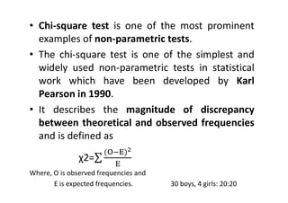
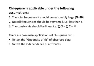
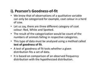
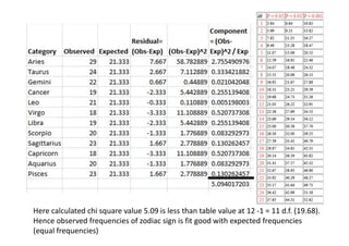
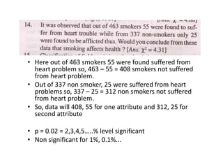
The document provides information on the Chi-Square test, a non-parametric test used to analyze categorical data. It discusses two main applications of the Chi-Square test: 1) testing goodness-of-fit of observed data to expected frequencies and 2) testing independence of attributes. Several examples are provided to demonstrate how to calculate the Chi-Square statistic and determine if the result is statistically significant based on the degrees of freedom and selected significance level.

1. Lecture 8
Chi Square Test
(Non Parametric Test)
Dr. Ashish. C. Patel
Assistant Professor,
Dept. of Animal Genetics & Breeding,
Veterinary College, Anand
STAT-531
Data Analysis using Statistical Packages

2. • There are basically two types of random variables and
they yield two types of data: numerical and categorical.
• Basically categorical variable yield data in the categories
and numerical variables yield data in numerical form.
• Responses to such questions as
"What is your major subject?" or
Do you have your own car?" are categorical because
they yield data such as “Diary Microbiology" or "no."
• In contrast, responses to such questions as "How tall
are you?" or "What is your G.P.A.?" are numerical.
• Numerical data can be either discrete or continuous.

3. • Discrete data arise from a counting process, while
continuous data arise from a measuring process.
• The Chi Square statistic compares the counts of
categorical responses between two (or more)
independent groups.
• (Note: Chi square tests can only be used on actual
numbers and not on percentages, proportions, means)

4. Non Parametric test: Chi-Squared test
• Various test of significance such as z, t and F are
based on the assumption that the samples are
drawn from the normally distributed populations.
• Since the testing procedure requires assumption
about the population values, these test are
known as parametric tests.
• There are many situations in which it is not
possible to make any assumption about the
population, from which the samples are drawn.
• Under these limitations alternative techniques
known as non-parametric tests have been
developed.

5. • Chi-square test is one of the most prominent
examples of non-parametric tests.
• The chi-square test is one of the simplest and
widely used non-parametric tests in statistical
work which have been developed by Karl
Pearson in 1990.
• It describes the magnitude of discrepancy
between theoretical and observed frequencies
and is defined as
χ2=
Where, O is observed frequencies and
E is expected frequencies. 30 boys, 4 girls: 20:20

6. Chi-square is applicable under the following
assumptions:
1. The total frequency N should be reasonably large (N>50)
2. No cell frequencies should be very small. i.e. less than 5.
3. The constraints should be linear i.e. = = N.
There are two main applications of chi-square test:
• To test the “Goodness-of-fit” of observed data
• To test the independence of attributes

7. i). Pearson’s Goodness-of-fit
• We know that of observations of a qualitative variable
can only be categorized for example, coat colour in a herd
of cow.
• Let us say, there are three different category of coat
colour: Red, White and Spotted.
• The result of the categorization would be count of the
numbers of animals falling in respective categories.
• This type of data must be analysed using a method called
test of goodness of fit.
• A test of goodness of fit tests whether a given
distribution fits a set of data.
• It is based on comparison of an observed frequency
distribution with the hypothesized distribution.

8. This expression of “Goodness-of-fit” may be
used to describe the ‘Fit’ of observed and
hypothetical frequencies.
• If the calculated chi-square value of chi square
is significant at 5% level of significance, we say
that the fit is poor one or observed
frequencies are not in accordance with the
hypothesis assumed and vice versa.
• In this way we see that chi square affords a
measure of the correspondence between the
fact and the theory.

9. • Example: 256 visual artists were surveyed to find out their
zodiac sign. The results were:
• Aries (29),
• Taurus (24),
• Gemini (22),
• Cancer (19),
• Leo (21),
• Virgo (18),
• Libra (19),
• Scorpio (20),
• Sagittarius (23),
• Capricorn (18),
• Aquarius (20),
• Pisces (23).
• Test the hypothesis that zodiac signs are evenly distributed
across visual artists.

10. Expected frequency = 256/12 = 21.333

14. Here calculated chi square value 5.09 is less than table value at 12 -1 = 11 d.f. (19.68).
Hence observed frequencies of zodiac sign is fit good with expected frequencies
(equal frequencies)

15. • Exercise .
• The expected proportions of white, brown and
mix coloured rabbits in a population are 0.36,
0.48 and 0.16 respectively. In a sample of 400
rabbits there were 140 white, 240 brown and 20
mix coloured. Are the proportions in that sample
of rabbits different than expected?
• The observed and expected frequencies are
presented in the following table:

16. • χ2= = + +
= 42.36
• The critical value of the chi-square distribution for
k – 1 = 2 degrees of freedom and significance level
of α = 0.05 is 5.991. Since the calculated χ2 is
greater than the critical value it can be concluded
that the sample is different from the population
with 0.05 level of significance.
Color Observed Expected
White 140 400*0.36=144
Brown 240 400*0.48= 192
Mix coloured 20 400*0.16= 64

17. Pearson’s Goodness-of-fit
(Testing goodness of fit for observed ratio with some
hypothetical / Scientifically derived ratio)
Characters Observed Freq Expected Freq
Magenta flower + Green stigma 120 217 x 9/16 =122.06
Magenta flower + Red stigma 48 217 x 3/16 = 40.69
Red flower + Green stigma 36 217 x 3/16 = 40.69
Red flower + Red stigma 13 217 x 1/16 = 13.56
Total 217 217

18. • Here the observed frequency 161, 59
• Expected freq. 220 x ¾ = 165, 220 x ¼ = 55

19. • ii). Test of independence of attributes
• One can test whether two or more attributes
are associated or not i.e. the attributes are
independent or dependent.
• 2*2 contingency tables: In this we have two
attributes each at two levels. The test of
independence of attributes has been illustrated
in exercise.
• Degree of freedom for m x n contingency table
is (m-1)*(n-1)
• For e.g. 3 x 3 contingency table = (3-1)*(3-1)
= 2 x 2 = 4

20. • Exercise 6: In an anti COVID-19 campaign,
Covaxin was administered to 812 persons out of
a total population of 3248. The number of
COVID-19 +ve and -ve cases is shown below:
Discuss the usefulness of Covaxin in controlling
COVID-19.
Vaccination Corona +ve Corona -ve Total
Covaxin 20 792 812
No Covaxin 220 2216 2436
Total 240 3008 3248

21. • Ho: Covaxin is not effective in controlling COVID 19
i.e. two attributes are independent
• Ha: Covaxin is effective in controlling COVID 19 i.e.
two attributes are dependent
•
• Test Statistics :
• χ2= with (r-1)(c-1) = d.f.
• We need expected frequencies
Vaccination Corona
+ve
Corona
-ve
Total
Covaxin a=20 b=792 812=R1
No Covaxin c=220 d=2216 2436=R2
Total 240= C1 3008=C2 3248=N

22. • The expected frequency corresponding to first row
and first column is determined as
• E11= = = 60
• Similarly, the expected frequency corresponding to
second row and first column is obtained as
• E21= = = 180
• The expected frequency corresponding to first row
and second column is obtained as
• E12 = = = 752
• The expected frequency corresponding to second
row and second column is obtained as
• E22 = = = 2256
Vaccination Corona
+ve
Corona
-ve
Total
Covaxin a=20 b=792 812=R1
No Covaxin c=220 d=2216 2436=R2
Total 240= C1 3008=C2 3248=N

23. O E (O-E)2 (O-E)2/E
20 60 1600 26.667
220 180 1600 8.889
792 752 1600 2.218
2216 2256 1600 0.709
Now, χ2 cal . is 26.667+8.889+2.218+0.709 = 38.39
As the cal. value of χ2 (38.393) at 1 d.f. is much higher
than table value of χ2 (3.84) at 5% level of significance,
the null hypothesis is rejected. Hence, COVAXIN is found
useful in controlling COVID 19 virus

24. • Alternative method of calculating χ2 using
direct formula
• In a contingency table with attributes A and B
each at two levels, χ2 can be calculated using
direct formula
• χ2 =
• χ2 = =
= 38.39

25. • Yate’s Correction
• One of the conditions for the application of χ2
test is that no cell frequency should be less than
5.
• In case of 2*2 contingency table if any cell
frequency is less than 5, Yate’s (1934) proposed a
correction which involves increase in observed
frequencies (fo) by ½ in two of cells and reduce fo
by ½ in two of cells, without changing the
marginal totals.
• Using the Yate’s correction χ2 is obtained as, χ2=
.

26. • Ho: Vaccine is not effective in controlling TB
i.e. two attributes are independent
• Ha: Vaccine is effective in controlling TB i.e.
two attributes are dependent

28. • Here out of 463 smokers 55 were found suffered from
heart problem so, 463 – 55 = 408 smokers not suffered
from heart problem.
• Out of 337 non smoker, 25 were suffered from heart
problems so, 337 – 25 = 312 non smokers not suffered
from heart problem.
• So, data will 408, 55 for one attribute and 312, 25 for
second attribute
• p = 0.02 = 2,3,4,5…..% level significant
• Non significant for 1%, 0.1%...

29. https://stats.libretexts.org/Bookshelves/Ancillary_Materials/02%3A_Interacti
ve_Statistics/36%3A__Chi-Square_Goodness_of_Fit_Test_Calculator