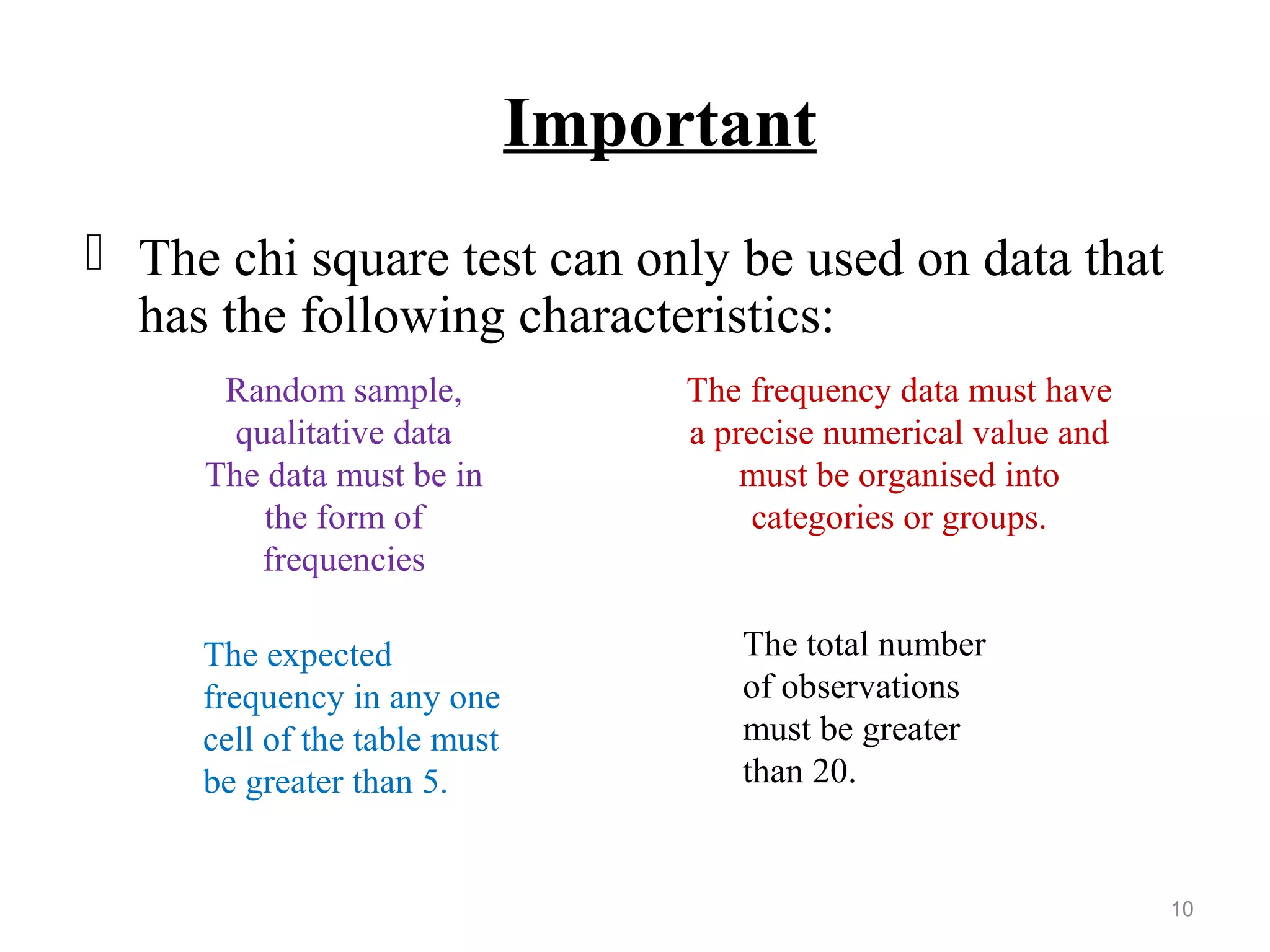
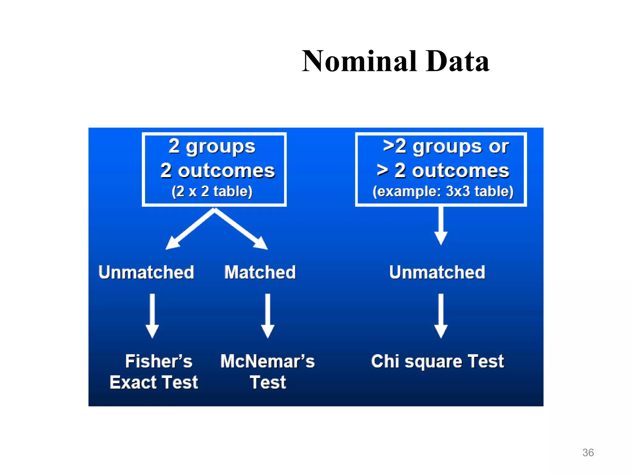
This document provides an overview of non-parametric statistical tests. It discusses tests such as the chi-square test, Wilcoxon signed-rank test, Mann-Whitney test, Friedman test, and median test. These tests can be used with ordinal or nominal data when the assumptions of parametric tests are not met. The document explains the appropriate uses and procedures for each non-parametric test.

1. Non-Parametric
Tests
Meenu Saharan
Ph.d Scholar(Pharmacology)
Guidance of:
Dr. Lokendra Sharma
Prof.Pharmacology
SMS Medical College, Jaipur
1

2. Tests of Significance
 Parametric tests
Students ‘t’ test
ANOVA
 Non Parametric tests
Chi square test
Wilcoxon’s signed rank test
Mann Whitney test
Friedman test
2

3. Four scales of measurement
Nominal :
Divided into qualitative categories e.g.
male/female, diseased/ non-diseased
Ordinal :
Placed in a meaningful order, E.g.1st
,2nd
,3rd
ranks
No information of size of interval
3

4. Four scales of measurement
Interval :
placed in a meaningful order
Have meaningful interval between the items
E.g. Celsius temperature scale
Do not have an absolute zero
Ratio :
Properties are same as interval
They have an absolute zero
E.g. BP in mmHg, HR
4

5. • Non parametric tests :
– Data doesn’t follow any specific distribution
– Discrete variables
– Ordinal / nominal measurements
5

6. How to pick the correct Stats ?
• What type of data is it ?
• How many number of comparison groups?
6

7. What is Matching?
 Observations or measurements made on the same
subject (or on individually matched subjects) are
said to be “matched” or “paired.”
 Examples:
Before and after measurements in the same
subject.
 Matching needs to be considered in selecting the
proper statistical test. 7

8. Nominal Data : Data which fits
into categories
 Binomial sample
 Sex: male / female
 Obese : yes / no
 Vaccinated or not vaccinated
e.g. 2x2 table
Chi square test
Fischer exact test
Mc Neamer test
8
 Multinomial samples
 Sample divided into > 2
categories
 E.g. diabetics and non-
diabetics
Grouped as weighing 40-
50 kg, 50-60 kg, 60-70 kg
and >70 kg
Chi square test

9. Chi Square Test
• Given by karl pearson
• Test of significance
• Used to measure the differences b/w what is observed
and what is expected according to an assumed
hypothesis
• To find diff b/w two proportions
• Test of association between two attributes eg:
smoking and lung cancer
9

10. Important
 The chi square test can only be used on data that
has the following characteristics:
10
Random sample,
qualitative data
The data must be in
the form of
frequencies
The frequency data must have
a precise numerical value and
must be organised into
categories or groups.
The expected
frequency in any one
cell of the table must
be greater than 5.
The total number
of observations
must be greater
than 20.

11. Example – trial of two whooping
cough vaccines
• Make contingency table of obsv frequencies
• Expected frequencies are calculated
• 1. Apply the null hypothesis i.e. No difference B/W two
vaccines
• 2. Pool the results
11
Vaccine Attacked Not attacked Total Attack rate
A 10(a) 90(b) 100 10%
B 26(c) 74(d) 100 26%
Total 36 164 200

12. • Proportion attacked = Total attacked
Total
= 36/200 = .18
• Proportion not attacked = Total not attacked
Total
= 164/200 = .82
12

13. For Vaccine A
Expected attacked = 100x36/200 = 18
Expected not attacked = 100x164/200 = 82
13
Expected frequency = row total x column total
total no in sample
For Vaccine B
Expected attacked = 100x36/200 = 18
Expected not attacked = 100x164/200 = 82

14. Rewriting the data
• = {(10 – 18)2
+ (90 - 82)2
+ (26 - 18)2
+ (74 -82)2
}
• 18 82 18 82
• = 64/18 + 64/82 + 64/18 + 64/82 = 8.670
• Calculate d.f. in 2 x 2 contingency table
• d.f. = (c-1)(r-1) = (2-1)(2-1) = 1
14
Vaccine Attacked Not attacked
A 0 = 10 0 = 90
E = 18 E = 80
B 0 = 26 0 = 74
E = 18 E = 82
χ 2
= ∑ (O – E)2
E

15. 15
So, x2
value (calculated) is highly significant at p <
0.005
Null hypothesis --- Rejected

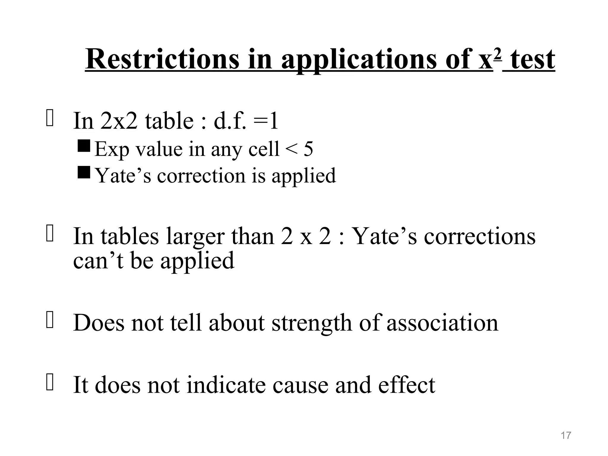
16. • If E frequency in any cell <5, Yates’ correction or
correction for continuity is applied
x2
= { [O - E] – 1/2 }2
E
16

17. Restrictions in applications of x2
test
 In 2x2 table : d.f. =1
Exp value in any cell < 5
Yate’s correction is applied
 In tables larger than 2 x 2 : Yate’s corrections
can’t be applied
 Does not tell about strength of association
 It does not indicate cause and effect
17

18. Wilcoxon’s Signed Rank Test
• For paired data
• Ex: differences in body wt in rats before & after an anorectic
compound have been recorded
• STEPS:
• Results are arranged in tabular form.
• Rank the diff in B.W. in increasing order, irrespective of sign
18

19.  Smallest value given rank 1
 Average ranks given
 Rank total : n(n+1)/2 ,n is no of items(rats)
 Respective sign is given to each rank
 Plus & minus ranks are added separately
 Smaller value taken for test of significance
 Irresptv of sign,tab of wilcxn on paired samples against no of pairs.
 Larger rank total,than tab are non significant
19

20. Ranking of differences in body wt in
each rat before & after treatment
20
Rat Diff in
B.W.(g)
Rank Rank Avg Signed
Rank
1 1 1 1 1
2 -2 2 2.5 -2.5
3 2 3 2.5 2.5
4 3 4 4 4
5 -4 5 5 -5
6 -7 6 6.5 -6.5
7 -7 7 6.5 -6.5
8 -9 8 8 -8
9 -11 9 9 -9
10 -12 10 10 -10

21.  Rank total = 55
 Plus ranks = 7.5
 Minus ranks = 47.5
 No. of paired obs = 1
 Smaller value 7.5 < tabulated value 8 at 5%
against 10 pairs
 So, result is significant at 5 %
21

22. Wilcoxon’s Two-sample Rank
Test
• Applied to unpaired samples
• STEPS:
• Obsv in both samples are combined into single & ranked in
order of magnitude
• Figures from one sample are distinguished from other by
underlining
22

23. • Example:
Number of jumps per mouse observed during
naloxone precipitated morphine withdrawal in control
and in atropine treated mice.
23

24. Number of jumps per mouse in
control & in treated group
24
Control mice No.of jumps Treated mice No.of jumps
1 5 1 15
2 2 2 9
3 13 3 11
4 6 4 5
5 5 5 31
6 8 6 36
7 2 7 9
8 5 8 18
9 9 9 23
10 17 10 21

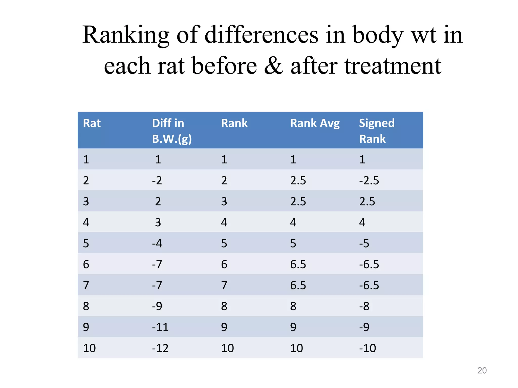
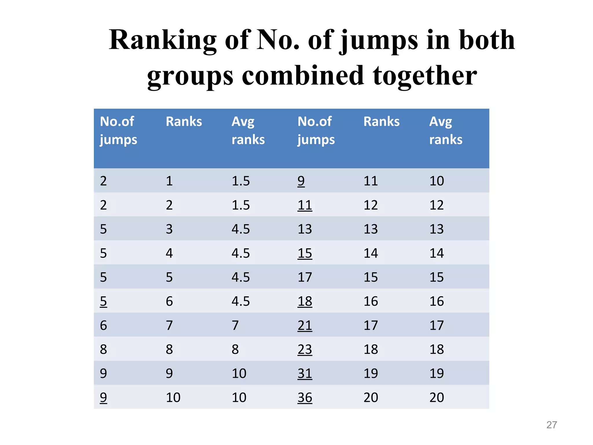
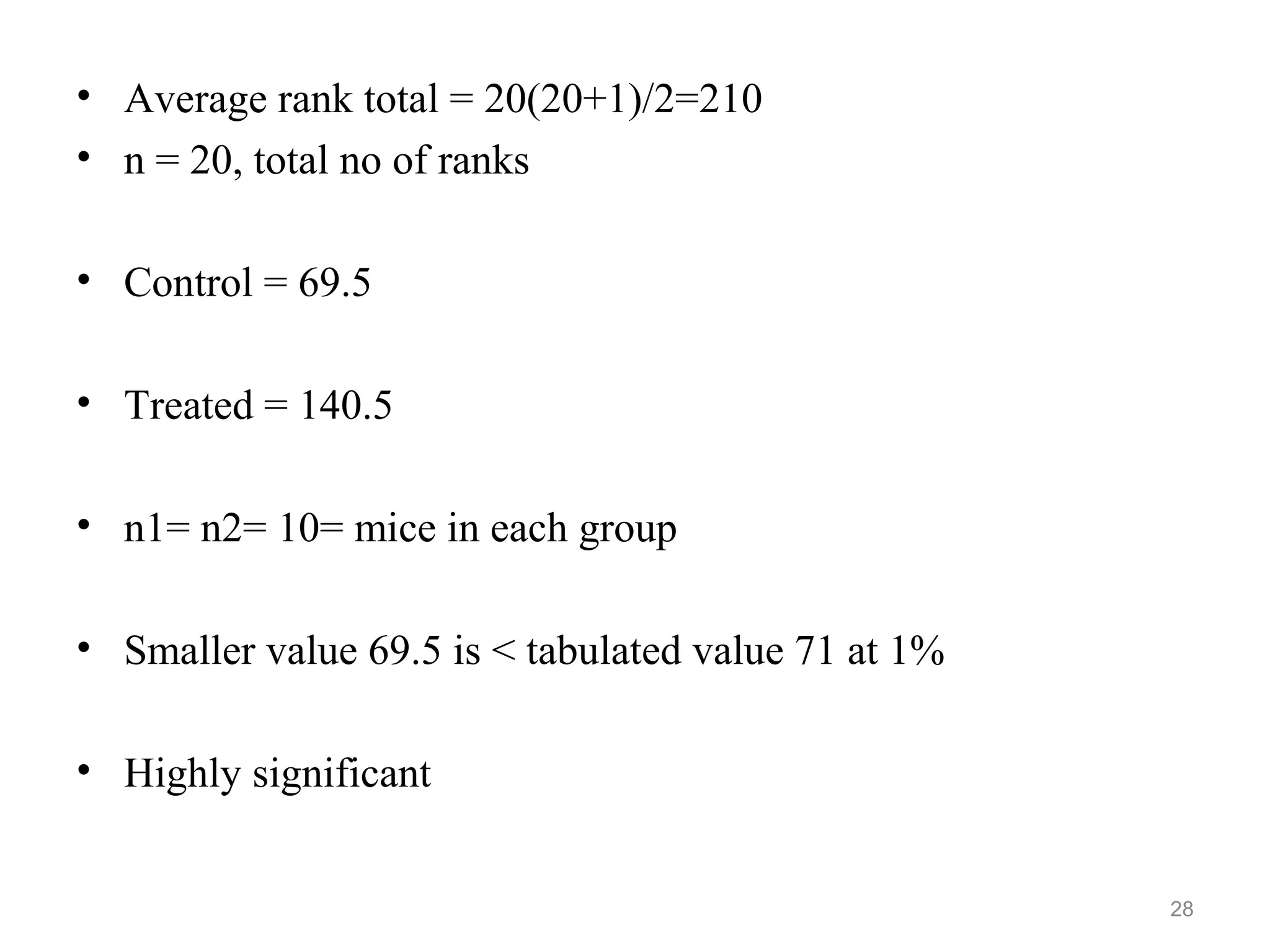
25. • Average ranks are given
• Rank total : n(n+1)/2 , n=total no of both samples
• Ranks of any one sample are added;
• If total(T1) > half the rank total of 2 samples together,
• Other rank total(T2) is calculated:
• T2 = [n(n+1)/2] – T1
• Smaller of two ranks is taken for test of significance
25

26. • Refer to tab of wilcoxon test on unpaired samples with
n1= no of obs in smaller sample
n2= no of obs in other sample
• If calculated value ≤ tabulated value: significant
• Reject the null hypothesis
26

27. Ranking of No. of jumps in both
groups combined together
27
No.of
jumps
Ranks Avg
ranks
No.of
jumps
Ranks Avg
ranks
2 1 1.5 9 11 10
2 2 1.5 11 12 12
5 3 4.5 13 13 13
5 4 4.5 15 14 14
5 5 4.5 17 15 15
5 6 4.5 18 16 16
6 7 7 21 17 17
8 8 8 23 18 18
9 9 10 31 19 19
9 10 10 36 20 20

28. • Average rank total = 20(20+1)/2=210
• n = 20, total no of ranks
• Control = 69.5
• Treated = 140.5
• n1= n2= 10= mice in each group
• Smaller value 69.5 is < tabulated value 71 at 1%
• Highly significant
28

29. Wilcoxon rank-sum test or
Wilcoxon–Mann–Whitney test)
 For assessing whether two independent samples
of observations have equally large values.
 One of the best-known non-parametric tests.
 Proposed initially by Frank Wilcoxonin 1945,
for equal sample sizes, and extended by H. B.
Mann and D. R. Whitney (1947).
Cont……
29

30. Wilcoxon rank-sum test or
Wilcoxon–Mann–Whitney test)
• MWW is virtually identical to performing an
parametric two-sample t test on the data after
ranking over the combined samples.
30

31. Median Test
 Special case of Pearson's chi-square test.
 Tests that the medians of the populations from
which two samples are drawn are identical.
 The data in each sample are assigned to two
groups, one consisting of data whose values
are higher than the median value in the two
groups combined
Cont……
31

32. Median Test
 and the other consisting of data whose values
are at the median or below.
 A Pearson's chi-square test is then used to
determine whether the observed frequencies
in each group differ from expected
frequencies derived from a distribution
combining the two groups.
32

33. McNemar’s Test
 Used on nominal data.
 It is applied to 2 × 2 contingency tables with
matched pairs of subjects
 Determine whether the row and column marginal
frequencies are equal
 It is named after Quinn McNemar, who
introduced it in 1947.
 An application of the test in genetics is the
transmission disequilibrium test for detecting
genetic linkage.
33

34. Friedman Test
• Developed by the U.S. economist Milton
Friedman.
• Similar to the parametric repeated measures
ANOVA
• Used to detect differences in treatments across
multiple test attempts.
• Involves ranking each row together, then
considering the values of ranks by columns.
34

35. Ordinal Data
35

36. Nominal Data
36

37. References
 Park’s Preventive& Social medicine;21st
ed
 Methods in Biostatistics,B K Mahajan;7th
ed
 Fundaments of Experimental Pharmacology,M N
Ghosh;4t ed
37

38. 38
Thank You