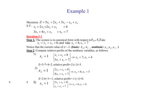
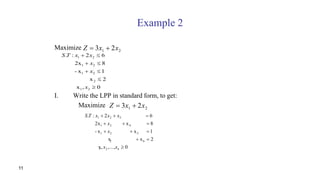
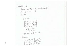
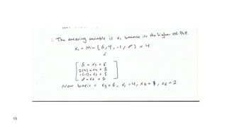
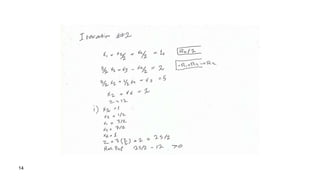
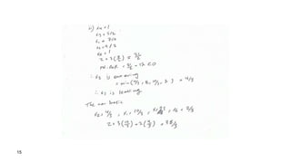
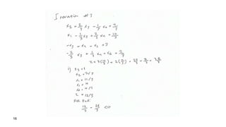
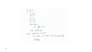
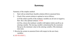
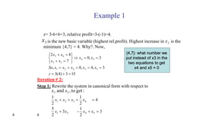
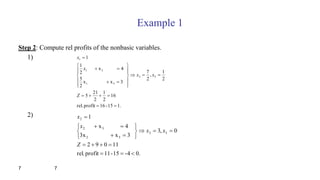
1. The simplex method is an iterative process for solving linear programming problems (LPPs) expressed in standard form. 2. It starts with an initial basic feasible solution (BFS) and improves the solution at each iteration by finding an adjacent BFS with a better objective value, until no further improvements can be made. 3. Each iteration involves computing the relative profits of non-basic variables to determine an entering variable, then rewriting the system in canonical form with respect to the new basic variables defined by the minimum ratio test.

1. Chapter 03 - The Simplex Method Principles

2. 2 2
The Simplex Method
Principles
Definition: A variable is said to a basic variable in a given equation if
it appears with a unit coefficient in that equation and zero coefficients in
all other equations.
Other variables are called nonbasic variables.
Remark: Recall the reduced row-echelon form of the augmented matrix
of a system of linear equations.
Definition: A pivot operation is a sequence of elementary operations
that reduces a given system to an equivalent system in which a specified
variable has a unit coefficient in one equation and zero elsewhere. (this
is a basic variable).
Example:
yields the system
After a sequence of elementary row operations. This is called the
canonical form of the system.
43
2242
54321
54321


xxxxx
xxxxx
232
6423
5432
5431


xxxx
xxxx

3. 3 3
The Simplex Method
Principles
Definition: A variable is said to be a basic variable in a given system of linear
equations if it appears with a unit coefficient in one equation and zero
coefficients in other equations. Other variables are called nonbasic variables.
Definition: A pivot operation is a sequence of elementary row operations that
reduces a given system to an equivalent system in which a specified variable
has a unit coefficient in one equation and zero elsewhere. (Basic variable).
Remark: The number of basic variables is determined by the number of equations
in the system. (no. of basic variables is less than or equal to the no. of
equations).
Definition: The solution obtained from a canonical system by setting the nonbasic
variables to zero and solving for the basic variables is called a basic solution.
A basic feasible solution is a basic solution in which the values of the basic
variables are all nonnegarive.
In the previous example, the basic feasible solution is
1x
.2xand6 21 x

4. 4 4
The Simplex Method
Principles
The simplex method is an iterative process for solving LPP’s expressed in
standard form . In addition to that, the constraint equations are expressed
in a canonical system.
Steps:
1. Start with an initial basic feasible solution in canonical form.
2. Improve the initial solution (if possible) by finding another bfs with a
better objective function value. The SM implicitly eliminates from
consideration all those bfs’s whose objective function values are worse
than the present (current) solution.
3. Continue until a particular bfs cannot be improved further. It becomes an
optimal solution, and the method terminates.
Definition: A bfs that differs from the present bfs by exactly one basic variable
is called an adjacent bfs.
Definition: The relative profit of a variable is the change in the value of the
objective function that results from increasing the value of this variable
by 1.

5. 5 5
Example 1
Maximize
S.T :
Iteration # 1
Step 1: The system is in canonical form with respect to . Take
Notice that the current value of z= -1. (basic: , nonbasic: )
Step 2: Compute relative profits of the nonbasic variables, as follows:
1)
Z=5-7+4=2, relative profit=2-(-1)=3.
2)
Z=2-6+3=-1, relative profit=-1-(-1)=0.
3)
54321 325 xxxxxZ 
7x43x
822
5321
4321


xx
xxxx
7,8takeand,0 54321  xxxxx
.,, 321 xxx
11 x
54 , xx
54 , xx
4,7
73
8
54
51
41









xx
xx
xx
12 x 3,6
74
82
54
52
42









xx
xx
xx
13 x 6,6
7
82
54
53
43









xx
xx
xx

6. 6 6
Example 1
z= 3-6+6=3, relative profit=3-(-1)=4.
is the new basic variable (highest rel.profit). Highest increase in is the
minimum {4,7} = 4. Why?. Now,
Iteration # 2:
Step 1: Rewrite the system in canonical form with respect to
3x 3x
153)4(3
3,4,0,
3,0
7
82
53421
54
53
43











z
xxxxxSo
xx
xx
xx
:getto,and 53 xx
3
2
1
-3
2
5
4
2
1
2
1
5421
4321


xxxx
xxxx
{4,7}: what number we
put instead of x3 in the
two equations to get
x4 and x5 = 0

7. 7 7
Example 1
Step 2: Compute rel profits of the nonbasic variables.
1)
2)
1.15-16profitrel.
16
2
1
2
21
5
2
1
,
2
7
3xx
2
5
4x
2
1
1
53
51
31
1


















Z
xx
x
x
0.-415-11profitrel.
11092
0,3
3x3x
4x
1
53
52
32
2












Z
xx
x
x

8. 8
Example 1
3)
is the new basic variable. = min{8,6/5} = 6/5.
0.-215-13profit.
13
2
7
1
2
21
2
7
,
2
7
3
2
1
4
2
1
1
53
54
43
4


















rel
Z
xx
xx
xx
x
1x 1x
  0x:nonbasic,,:
5
81
5
51
6
5
17
5
3
4
54213
3



xxxxbasic
Z
x

9. 9
Example 1
Iteration # 3
Step 1: Rewrite the system in canonical form with respect to
1)
2)
:getto,and 31 xx
5
17
5
1
5
3
x
5
2
5
6
x
5
2
5
1
-
5
6
5432
5421


xxx
xxx
03
5
15
5
81
11.,1192
3,0
5
17
5
2
5
6
5
6
1
31
32
21
2

















profitrelZ
xx
xx
xx
x
03
5
9
5
81
5
72
.,
5
72
1
5
42
7
5
14
,
5
7
5
17
5
3
5
6
5
1
1
31
43
41
4

















profitrelZ
xx
xx
xx
x

10. 10
Example 1
3)
Conclusion: All relative profits in this iteration are negative. Therefore,
there is no new entering variables. The results of the previous iteration
give the optimal solution. i.e
DONE
0
5
2
5
81
5
79
.,
5
79
1
5
54
4
5
18
,
5
4
5
17
5
1
5
6
5
2
1
31
53
51
5

















profitrelZ
xx
xx
xx
x
5
81
,
5
17
,
5
6
31  Zxx

11. 11
Example 2
Maximize
I. Write the LPP in standard form, to get:
Maximize
21 23 xxZ 
0,x
2x
1x-
82x
62:.
21
2
21
21
21





x
x
x
xxTS
21 23 xxZ 
0,...,,x
2xx
1xx-
8x2x
62:.
621
62
521
421
321





xx
x
x
xxxTS

12. 12
Example 2

13. 13

14. 14

15. 15

16. 16

17. 17

18. Summary
Summary of the simplex method:
1. Start with an initial basic feasible solution (bfs) in canonical form.
2. Check if the current solution is optimal or not as follows:
(i) If the relative profits of the nonbasic variables are all zero or negative,
then this is the optimal solution. STOP.
(ii) Else, choose the nonbasic variable with highest relative profit as an
entering variable. The leaving variable is determined by the constraint
that gives the minimum value to the entering variable. (The minimum
ratio rule).
3. Rewrite the system in canonical form with respect to the new basic
variables.
4. GO TO STEP 2.