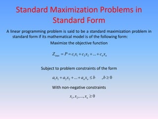
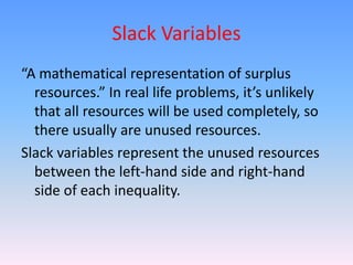
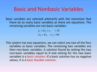
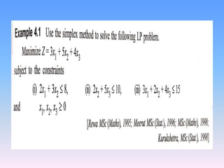
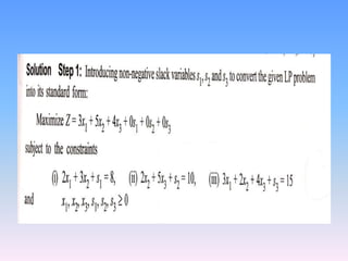
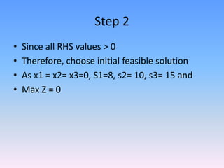
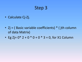
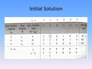
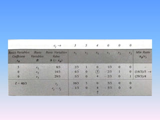
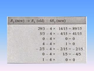
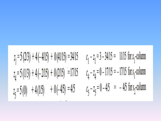
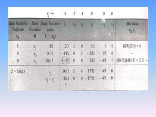
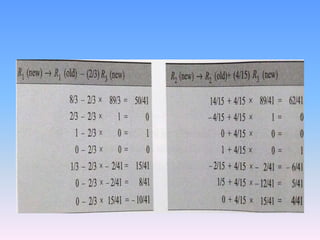
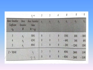
The Simplex Method
The geometric method of solving linear programming problems
presented before. The graphical method is useful only for
problems involving two decision variables and relatively few
problem constraints.
What happens when we need more decision variables and more problem constraints?
We use an algebraic method called the simplex method, which
was developed by George B. DANTZIG (1914-2005) in 1947 while
on assignment with the U.S. Department of the air force.
Standard Maximization Problems in
Standard Form
A linear programming problem is said to be a standard maximization problem in
standard form if its mathematical model is of the following form:
Maximize the objective function
Subject to problem constraints of the form
With non-negative constraints
max 1 1 2 2 ... n n
Z P c x c x c x
    
1 1 2 2 ... , 0
n n
a x a x a x b b
    
1 2
, ,..., 0
n
x x x 
Slack Variables
“A mathematical representation of surplus
resources.” In real life problems, it’s unlikely
that all resources will be used completely, so
there usually are unused resources.
Slack variables represent the unused resources
between the left-hand side and right-hand
side of each inequality.
Basic and Nonbasic Variables
Basic variables are selected arbitrarily with the restriction that
there be as many basic variables as there are equations. The
remaining variables are non-basic variables.
This system has two equations, we can select any two of the four
variables as basic variables. The remaining two variables are
then non-basic variables. A solution found by setting the two
non-basic variables equal to 0 and solving for the two basic
variables is a basic solution. If a basic solution has no negative
values, it is a basic feasible solution.
1 2 1
1 2 2
2 32
3 4 84
x x s
x x s
  
  
Step 2
• Since all RHS values > 0
• Therefore, choose initial feasible solution
• As x1 = x2= x3=0, S1=8, s2= 10, s3= 15 and
• Max Z = 0
Step 3
• Calculate Cj-Zj.
• Zj = ( Basic variable coefficients) * ( jth column
of data Matrix)
• Eg Zj= 0* 2 + 0 * 0 + 0 * 3 = 0, for X1 Column
Initial Solution
Step 4
• The variable that is to leave the basis is
determined by dividing the values in XB
column by the corresponding elements in the
key column
• Iteration 2- repeat Step 3 to 5
• Iteration 3
simplex method
simplex method

simplex method

  • 1.
    The Simplex Method Thegeometric method of solving linear programming problems presented before. The graphical method is useful only for problems involving two decision variables and relatively few problem constraints. What happens when we need more decision variables and more problem constraints? We use an algebraic method called the simplex method, which was developed by George B. DANTZIG (1914-2005) in 1947 while on assignment with the U.S. Department of the air force.
  • 2.
    Standard Maximization Problemsin Standard Form A linear programming problem is said to be a standard maximization problem in standard form if its mathematical model is of the following form: Maximize the objective function Subject to problem constraints of the form With non-negative constraints max 1 1 2 2 ... n n Z P c x c x c x      1 1 2 2 ... , 0 n n a x a x a x b b      1 2 , ,..., 0 n x x x 
  • 3.
    Slack Variables “A mathematicalrepresentation of surplus resources.” In real life problems, it’s unlikely that all resources will be used completely, so there usually are unused resources. Slack variables represent the unused resources between the left-hand side and right-hand side of each inequality.
  • 4.
    Basic and NonbasicVariables Basic variables are selected arbitrarily with the restriction that there be as many basic variables as there are equations. The remaining variables are non-basic variables. This system has two equations, we can select any two of the four variables as basic variables. The remaining two variables are then non-basic variables. A solution found by setting the two non-basic variables equal to 0 and solving for the two basic variables is a basic solution. If a basic solution has no negative values, it is a basic feasible solution. 1 2 1 1 2 2 2 32 3 4 84 x x s x x s      
  • 7.
    Step 2 • Sinceall RHS values > 0 • Therefore, choose initial feasible solution • As x1 = x2= x3=0, S1=8, s2= 10, s3= 15 and • Max Z = 0
  • 8.
    Step 3 • CalculateCj-Zj. • Zj = ( Basic variable coefficients) * ( jth column of data Matrix) • Eg Zj= 0* 2 + 0 * 0 + 0 * 3 = 0, for X1 Column
  • 9.
  • 10.
    Step 4 • Thevariable that is to leave the basis is determined by dividing the values in XB column by the corresponding elements in the key column
  • 14.
    • Iteration 2-repeat Step 3 to 5
  • 18.