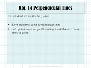
Obj. 14 Perpendicular Lines
•
0 likes•1,853 views
Solve problems using perpendicular lines Set up and solve inequalities using the distance from a point to a line
Report
Share
Report
Share
Download to read offline

Recommended
1.4.4 Parallel and Perpendicular Line Equations
Use slopes to identify parallel and perpendicular lines.
Write equations of line parallel or perpendicular to a given line through a given point.
1.4.3 Slopes and Equations of Lines
The document discusses slopes and equations of lines. It defines slope as the ratio of the rise to the run between two points on a line. It explains how to find the slope from two points, a graph, or an equation. It also explains how to write the equation of a line in point-slope form, slope-intercept form, or for horizontal and vertical lines. Examples are provided for finding slopes and writing equations in different forms.
2.8.5 Coordinate Plane Quads
This document discusses classifying quadrilaterals based on their coordinates. It explains that to identify special types of quadrilaterals like parallelograms, rectangles, rhombi, squares, trapezoids, and kites, one can use the distance and slope formulas to determine if sides are parallel or congruent. An example problem demonstrates using the formulas to show a quadrilateral with given coordinates is a square.
2.8.4 Kites and Trapezoids
This document discusses properties of kites and trapezoids. It defines kites as quadrilaterals with two pairs of congruent consecutive nonparallel sides, and notes their diagonals are perpendicular. It defines trapezoids as quadrilaterals with one pair of parallel sides called bases, and notes angles along the legs are supplementary. It provides theorems about isosceles trapezoids having congruent base angles or congruent diagonals. It also states the midsegment theorem for trapezoids.
Analytical geometry
This document discusses analytical geometry concepts including finding the distance between two points using the distance formula, calculating the gradient of a line, identifying properties of straight lines including their standard and alternate forms, characteristics of parallel and perpendicular lines including their gradient relationships, and the formula to find the midpoint between two points on a line.
1.3.2C Equations of Lines
* Find the slope of a line.
* Use slopes to identify parallel and perpendicular lines.
* Write the equation of a line through a given point
- parallel to a given line
- perpendicular to a given line
Optimum polygon triangulation
The document discusses optimal triangulation of convex polygons. It defines key terms like polygon, convex polygon, chords, and triangulation. It states that the optimal polygon triangulation problem is to find a triangulation that minimizes the sum of weights of triangles, where weight could be triangle side lengths. The problem is similar to matrix chain multiplication, as both can be viewed as parse trees, and the matrix problem can be modified to solve triangulation.
Sol50
The document describes a method for inductively dividing a line segment into an increasing number of equal parts. It starts with a segment divided into three equal parts and shows how to add one more division point to create four equal parts. This is done by drawing lines from an arbitrary point P through the existing division points and their intersections with a parallel line L. Similar triangle ratios are used to prove the new division points bisect the original segment lengths, creating four equal parts. The method can be repeated to divide the segment into any number of equal parts.
Stragiht lines (2020 21)
This document discusses slope and how to calculate it. It defines slope as the ratio of the rise over the run between two points on a line. A vertical line has an undefined slope since the run is zero. For a non-vertical line, the slope is calculated as the change in y-values divided by the change in x-values between two points. The slope indicates whether the line rises or falls from left to right. An example demonstrates how to sketch a line given its slope and a point.
Curve tracing
Polar coordinates represent points in a plane using an ordered pair (r, θ) where r is the distance from a fixed point called the pole (or origin) and θ is the angle between the line from the pole to the point and a reference axis called the polar axis. Some key properties:
- Points (r, θ) and (-r, θ + π) represent the same location.
- Polar equations like r = a describe circles with radius a centered at the pole.
- Equations can be converted between Cartesian (x, y) and polar (r, θ) coordinates using trigonometric relationships.
- Graphs of polar equations r = f(θ) consist of all points satisfying
TRACING OF CURVE (CARTESIAN AND POLAR)
This document discusses procedures for tracing polar curves. It explains how to determine symmetry properties, the region over which the curve is defined, tabulation of points, finding the angle between the radius vector and tangent, and identifying asymptotes. Two examples are provided to demonstrate the tracing process. The first example traces the curve r=a(1+cosθ) and finds it is symmetric about the initial line, lies within a circle, and passes through the origin. The second example traces r2=a2cos2θ, finding its symmetries and that the curve exists between 0<θ<π/4 and 3π/4<θ<π.
Graph of a linear equation vertical lines
- The document discusses graphing linear equations where a = 1 and b = 0, which produces a vertical line.
- It shows that the equation 1x + 0y = c is equivalent to x = c, and the graph of x = c is a vertical line passing through the point (c, 0).
- It concludes that for any equation of the form ax + by = c, where a = 1 and b = 0, the graph will be a vertical line.
Lesson 13 algebraic curves
1) The document defines algebraic curves as geometric figures formed by the set of points satisfying a given equation relating x and y.
2) Key properties of algebraic curves include their extent (domain and range), symmetry, intercepts, and asymptotes. Symmetry can be tested by substituting -x or -y. Intercepts are where the curve crosses the axes. Asymptotes are lines a curve approaches but never touches.
3) Tracing a curve involves determining its region, testing for symmetry, finding intercepts and asymptotes, and plotting points to sketch the curve.
3º mat pc_e_03_septiembre-alumno
1. The document is a math workbook covering tangent and normal lines to curves. It reviews the definition of the derivative and the equation of a tangent line.
2. It defines a normal line as perpendicular to the tangent line and gives the condition for perpendicular lines as having slopes that are negative reciprocals of each other.
3. It provides examples of finding the equations of tangent and normal lines for different curves at given points and representing them graphically.
January 16, 2015
- The document outlines notes on slope and linear equations from a class. It includes definitions of slope, formulas for calculating slope between two points, and examples of finding the slope and equation of a line from graphical data or given information.
- Students will review slope formulas, work examples and practice problems, and complete class work 2.11 applying concepts of slope and linear equations. The notes provide guidance on finding slope, writing equations of lines in slope-intercept and standard form, and graphing lines on coordinate planes.
Presentation on inverse matrix
This document discusses inverse matrices and methods for calculating them. It defines an inverse matrix as a matrix M-1 such that MM-1=M-1M=I, where I is the identity matrix. Only square matrices can have inverses. Two common methods for calculating the inverse are Crammer's Method, which uses the adjoint and determinant of the matrix, and Gauss Method, which performs row operations. An example calculates the inverse of a 2x2 matrix using the property that the inverse is the transpose of the cofactor matrix divided by the determinant.
Graphing Linear Inequalities
- A linear inequality describes a region of the coordinate plane bounded by a line. Any point in the shaded region is a solution to the inequality.
- To graph a linear inequality, first solve it for y and graph the resulting equation as a line. Then, test a point not on the line to determine which side of the line to shade based on whether it satisfies the inequality.
- The line is drawn solid for ≤ or ≥ and dashed for < or >. Shading the correct side of the line indicates the full solution set of the inequality.
11.6 graphing linear inequalities in two variables
This document discusses how to graph linear inequalities in two variables. It provides examples of graphing various inequalities, including 2x + 3y ≤ 6, 2x + y > 3, and y < 3x. The process involves graphing the boundary line defined by the equal case of the inequality and then shading the appropriate region based on checking if a test point satisfies the inequality. Key steps are to draw the boundary line as solid or dashed based on the symbols (< or > versus ≤ or ≥) and then shade the region containing points that satisfy the inequality.
Differential Calculus
This document discusses various topics related to differential calculus including:
1. Envelopes and families of curves defined by equations of the form F(x,y,a)=0 where the parameter a defines each curve.
2. Asymptotes of curves, including vertical, horizontal, and oblique asymptotes.
3. Methods for finding the slopes and equations of asymptotes for algebraic curves, which involve putting the curve in terms of its highest degree terms and setting the results equal to 0.
4. Examples showing how to apply these methods to find the asymptotes of a specific algebraic curve.
1.3 SYMMETRY
The document discusses three types of symmetry for graphs: x-axis symmetry, where (x,y) corresponds to (x,-y); y-axis symmetry, where (x,y) corresponds to (-x,y); and origin symmetry, where (x,y) corresponds to (-x,-y). It provides tests for each type of symmetry by replacing variables in the graphing equation. An example at the end finds no x-axis or origin symmetry but y-axis symmetry.
7.2 Similar Polygons
The student is able to identify scale factors and use them to solve problems involving similar polygons. Scale factors allow comparison of corresponding side lengths of similar polygons through proportions. To determine if two polygons are similar, their corresponding angles must be congruent and side lengths must be proportional as shown through equal ratios.
Straight lines
The document presents information about straight lines and coordinates systems. It discusses key concepts such as the Cartesian coordinate system developed by Rene Descartes, which specifies each point in a plane using perpendicular x and y axes. The document also covers the definition of a straight line as the shortest distance between two points, midpoint and centroid formulas, polar coordinates, slope as a measure of a line's steepness, and the general equation of a straight line. The presentation is delivered to a lecturer by five students who each discuss different aspects of straight lines and coordinate systems.
1.4.4 Parallel and Perpendicular Line Equations
Use slopes to identify parallel and perpendicular lines
Write equations of a line parallel or perpendicular to a given line through a given point.
8004 side splitter 2013
The document discusses several theorems related to proportionality in triangles:
- The side-splitter theorem states that a line parallel to one side of a triangle divides the other two sides proportionally.
- The triangle proportionality theorem can be used to verify if two segments are parallel.
- The two transversal proportionality corollary states that two or more parallel lines divide two transversals proportionally.
- The triangle angle bisector theorem states that if a ray bisects an angle of a triangle, it divides the opposite side into segments proportional to the other two sides. Examples are provided to demonstrate applying these theorems.
Introduction to engineering maths
This document provides an introduction and overview of key concepts in mathematics that are important for engineering, including algebra, geometry, trigonometry, and calculus. It defines each area of math and outlines prerequisites. Algebra concepts like properties of equality, exponents, polynomials, and solving equations are explained. The document also covers lines and their standard form, noting that slope indicates whether a line rises or falls and what a zero slope represents. The overall goal is to help students understand what each math concept involves and how they are applied in engineering problems.
Polar Graphs: Limaçons, Roses, Lemniscates, & Cardioids
Learn about different polar graphs, including limaçons (convex, dimpled, looped), lemniscates, rose curves, and cardioids. View compare and contrast between the 4 different types of polar graphs, and view my impressions on this final unit in pre-calculus honors.
1.4.3 Slopes and Equations of Lines
The document discusses slopes and equations of lines. It defines slope as rise over run and explains how to calculate slope from two points on a line or from the graph of a line. It also explains how to write the equation of a line in point-slope form, slope-intercept form, or for horizontal and vertical lines. Several examples are provided of finding slopes and writing line equations in different forms.
Straight Lines for JEE REVISION Power point presentation
The document provides information about the weightage and number of problems on straight lines that have been asked in JEE Main from 2020-2024. It lists important subtopics of straight lines like locus of a point, reflection, pair of lines, etc. It also provides various important formulas related to straight lines, short notes, and sample problems related to important subtopics. The document is a comprehensive reference material for the straight lines chapter of JEE Main exam preparation.
Perpendicular lines, gradients, IB SL Mathematics
Here are the steps to solve these problems:
1. Find the slopes of the two lines:
m1 = (8-2)/(5--2) = 6/3 = 2 (slope of r)
m2 = (7-0)/(-8--2) = 7/-6 = -1 (slope of s)
The slopes are negative reciprocals, so r ⊥ s.
2. The slopes are m1 = 2 and m2 = -1/2. Since m1 × m2 = -1, the lines are perpendicular.
3. The given line has slope 3. The perpendicular line will have slope -1/3. Plug into the point-slope form
Straight Lines ( Especially For XI )
This is a document based on straight lines specially for XI Std. This is based on its various forms of equations, Formula.
More Related Content
What's hot
Stragiht lines (2020 21)
This document discusses slope and how to calculate it. It defines slope as the ratio of the rise over the run between two points on a line. A vertical line has an undefined slope since the run is zero. For a non-vertical line, the slope is calculated as the change in y-values divided by the change in x-values between two points. The slope indicates whether the line rises or falls from left to right. An example demonstrates how to sketch a line given its slope and a point.
Curve tracing
Polar coordinates represent points in a plane using an ordered pair (r, θ) where r is the distance from a fixed point called the pole (or origin) and θ is the angle between the line from the pole to the point and a reference axis called the polar axis. Some key properties:
- Points (r, θ) and (-r, θ + π) represent the same location.
- Polar equations like r = a describe circles with radius a centered at the pole.
- Equations can be converted between Cartesian (x, y) and polar (r, θ) coordinates using trigonometric relationships.
- Graphs of polar equations r = f(θ) consist of all points satisfying
TRACING OF CURVE (CARTESIAN AND POLAR)
This document discusses procedures for tracing polar curves. It explains how to determine symmetry properties, the region over which the curve is defined, tabulation of points, finding the angle between the radius vector and tangent, and identifying asymptotes. Two examples are provided to demonstrate the tracing process. The first example traces the curve r=a(1+cosθ) and finds it is symmetric about the initial line, lies within a circle, and passes through the origin. The second example traces r2=a2cos2θ, finding its symmetries and that the curve exists between 0<θ<π/4 and 3π/4<θ<π.
Graph of a linear equation vertical lines
- The document discusses graphing linear equations where a = 1 and b = 0, which produces a vertical line.
- It shows that the equation 1x + 0y = c is equivalent to x = c, and the graph of x = c is a vertical line passing through the point (c, 0).
- It concludes that for any equation of the form ax + by = c, where a = 1 and b = 0, the graph will be a vertical line.
Lesson 13 algebraic curves
1) The document defines algebraic curves as geometric figures formed by the set of points satisfying a given equation relating x and y.
2) Key properties of algebraic curves include their extent (domain and range), symmetry, intercepts, and asymptotes. Symmetry can be tested by substituting -x or -y. Intercepts are where the curve crosses the axes. Asymptotes are lines a curve approaches but never touches.
3) Tracing a curve involves determining its region, testing for symmetry, finding intercepts and asymptotes, and plotting points to sketch the curve.
3º mat pc_e_03_septiembre-alumno
1. The document is a math workbook covering tangent and normal lines to curves. It reviews the definition of the derivative and the equation of a tangent line.
2. It defines a normal line as perpendicular to the tangent line and gives the condition for perpendicular lines as having slopes that are negative reciprocals of each other.
3. It provides examples of finding the equations of tangent and normal lines for different curves at given points and representing them graphically.
January 16, 2015
- The document outlines notes on slope and linear equations from a class. It includes definitions of slope, formulas for calculating slope between two points, and examples of finding the slope and equation of a line from graphical data or given information.
- Students will review slope formulas, work examples and practice problems, and complete class work 2.11 applying concepts of slope and linear equations. The notes provide guidance on finding slope, writing equations of lines in slope-intercept and standard form, and graphing lines on coordinate planes.
Presentation on inverse matrix
This document discusses inverse matrices and methods for calculating them. It defines an inverse matrix as a matrix M-1 such that MM-1=M-1M=I, where I is the identity matrix. Only square matrices can have inverses. Two common methods for calculating the inverse are Crammer's Method, which uses the adjoint and determinant of the matrix, and Gauss Method, which performs row operations. An example calculates the inverse of a 2x2 matrix using the property that the inverse is the transpose of the cofactor matrix divided by the determinant.
Graphing Linear Inequalities
- A linear inequality describes a region of the coordinate plane bounded by a line. Any point in the shaded region is a solution to the inequality.
- To graph a linear inequality, first solve it for y and graph the resulting equation as a line. Then, test a point not on the line to determine which side of the line to shade based on whether it satisfies the inequality.
- The line is drawn solid for ≤ or ≥ and dashed for < or >. Shading the correct side of the line indicates the full solution set of the inequality.
11.6 graphing linear inequalities in two variables
This document discusses how to graph linear inequalities in two variables. It provides examples of graphing various inequalities, including 2x + 3y ≤ 6, 2x + y > 3, and y < 3x. The process involves graphing the boundary line defined by the equal case of the inequality and then shading the appropriate region based on checking if a test point satisfies the inequality. Key steps are to draw the boundary line as solid or dashed based on the symbols (< or > versus ≤ or ≥) and then shade the region containing points that satisfy the inequality.
Differential Calculus
This document discusses various topics related to differential calculus including:
1. Envelopes and families of curves defined by equations of the form F(x,y,a)=0 where the parameter a defines each curve.
2. Asymptotes of curves, including vertical, horizontal, and oblique asymptotes.
3. Methods for finding the slopes and equations of asymptotes for algebraic curves, which involve putting the curve in terms of its highest degree terms and setting the results equal to 0.
4. Examples showing how to apply these methods to find the asymptotes of a specific algebraic curve.
1.3 SYMMETRY
The document discusses three types of symmetry for graphs: x-axis symmetry, where (x,y) corresponds to (x,-y); y-axis symmetry, where (x,y) corresponds to (-x,y); and origin symmetry, where (x,y) corresponds to (-x,-y). It provides tests for each type of symmetry by replacing variables in the graphing equation. An example at the end finds no x-axis or origin symmetry but y-axis symmetry.
7.2 Similar Polygons
The student is able to identify scale factors and use them to solve problems involving similar polygons. Scale factors allow comparison of corresponding side lengths of similar polygons through proportions. To determine if two polygons are similar, their corresponding angles must be congruent and side lengths must be proportional as shown through equal ratios.
Straight lines
The document presents information about straight lines and coordinates systems. It discusses key concepts such as the Cartesian coordinate system developed by Rene Descartes, which specifies each point in a plane using perpendicular x and y axes. The document also covers the definition of a straight line as the shortest distance between two points, midpoint and centroid formulas, polar coordinates, slope as a measure of a line's steepness, and the general equation of a straight line. The presentation is delivered to a lecturer by five students who each discuss different aspects of straight lines and coordinate systems.
1.4.4 Parallel and Perpendicular Line Equations
Use slopes to identify parallel and perpendicular lines
Write equations of a line parallel or perpendicular to a given line through a given point.
8004 side splitter 2013
The document discusses several theorems related to proportionality in triangles:
- The side-splitter theorem states that a line parallel to one side of a triangle divides the other two sides proportionally.
- The triangle proportionality theorem can be used to verify if two segments are parallel.
- The two transversal proportionality corollary states that two or more parallel lines divide two transversals proportionally.
- The triangle angle bisector theorem states that if a ray bisects an angle of a triangle, it divides the opposite side into segments proportional to the other two sides. Examples are provided to demonstrate applying these theorems.
Introduction to engineering maths
This document provides an introduction and overview of key concepts in mathematics that are important for engineering, including algebra, geometry, trigonometry, and calculus. It defines each area of math and outlines prerequisites. Algebra concepts like properties of equality, exponents, polynomials, and solving equations are explained. The document also covers lines and their standard form, noting that slope indicates whether a line rises or falls and what a zero slope represents. The overall goal is to help students understand what each math concept involves and how they are applied in engineering problems.
Polar Graphs: Limaçons, Roses, Lemniscates, & Cardioids
Learn about different polar graphs, including limaçons (convex, dimpled, looped), lemniscates, rose curves, and cardioids. View compare and contrast between the 4 different types of polar graphs, and view my impressions on this final unit in pre-calculus honors.
1.4.3 Slopes and Equations of Lines
The document discusses slopes and equations of lines. It defines slope as rise over run and explains how to calculate slope from two points on a line or from the graph of a line. It also explains how to write the equation of a line in point-slope form, slope-intercept form, or for horizontal and vertical lines. Several examples are provided of finding slopes and writing line equations in different forms.
What's hot (19)
11.6 graphing linear inequalities in two variables
11.6 graphing linear inequalities in two variables
Polar Graphs: Limaçons, Roses, Lemniscates, & Cardioids
Polar Graphs: Limaçons, Roses, Lemniscates, & Cardioids
Similar to Obj. 14 Perpendicular Lines
Straight Lines for JEE REVISION Power point presentation
The document provides information about the weightage and number of problems on straight lines that have been asked in JEE Main from 2020-2024. It lists important subtopics of straight lines like locus of a point, reflection, pair of lines, etc. It also provides various important formulas related to straight lines, short notes, and sample problems related to important subtopics. The document is a comprehensive reference material for the straight lines chapter of JEE Main exam preparation.
Perpendicular lines, gradients, IB SL Mathematics
Here are the steps to solve these problems:
1. Find the slopes of the two lines:
m1 = (8-2)/(5--2) = 6/3 = 2 (slope of r)
m2 = (7-0)/(-8--2) = 7/-6 = -1 (slope of s)
The slopes are negative reciprocals, so r ⊥ s.
2. The slopes are m1 = 2 and m2 = -1/2. Since m1 × m2 = -1, the lines are perpendicular.
3. The given line has slope 3. The perpendicular line will have slope -1/3. Plug into the point-slope form
Straight Lines ( Especially For XI )
This is a document based on straight lines specially for XI Std. This is based on its various forms of equations, Formula.
Calculus academic journal (sample)
1. The document discusses techniques for finding extrema of functions, including absolute and local extrema. Critical points, endpoints, and the first and second derivative tests are covered.
2. The mean value theorem and Rolle's theorem are summarized. The mean value theorem relates the average and instantaneous rates of change over an interval.
3. Optimization problems can be solved by setting the derivative of the objective function equal to zero to find critical points corresponding to maxima or minima.
4. Newton's method is presented as an iterative process for approximating solutions to equations, using tangent lines to generate a sequence of improving approximations.
5. Anti-derivatives are defined as functions whose derivatives are a given
Share straight lines Presentation (3).pptx
This is actually a demonstration of the straight lines. This would be really helpful for the students of 11th standard. Though my presentation may not be fully clear, it definitely covers the main concepts associated with this topic. So students, I would be happy if this can be of any help to you all....thank you so much😊😊
R lecture co2_math 21-1
Discuss comprehensively the fundamental concepts in Analytic Geometry and use them to solve application problems and problems involving lines.
Vectors2
The document discusses various topics related to vectors and planes:
1. It explains the vector product in three forms - mathematical calculation, 3D picture, and in terms of sine. It provides an example to calculate the vector product of two vectors.
2. It discusses the different forms of the equation of a plane - parametric, scalar product, and Cartesian forms. It provides examples to write the equation of a plane in these different forms.
3. It explains how to find the foot of the perpendicular from a point to a plane. It provides examples to find the foot and shortest distance.
4. It discusses how to find acute angles between lines, planes, and a line and plane. Examples
Analytical geometry slides
The document discusses equations of lines, including:
1) The gradient-point form of a straight line equation which uses the gradient and coordinates of one point to determine the equation.
2) Calculating the gradient from two points on a line and using it to find the angle of inclination.
3) Determining the equation of a line parallel to another line, by setting their gradients equal since parallel lines have the same gradient.
Lecture 6
This document discusses singular value decomposition (SVD) and its applications. SVD decomposes a matrix into three component matrices that reveal useful properties about the matrix's structure and rank. SVD can be used to find the best-fitting line to a set of points by minimizing the sum of squared distances between points and the line. The solution involves computing the SVD of a transformed matrix and taking the right singular vector corresponding to the second largest singular value.
JC Vectors summary
1. The document provides revision on various topics in vectors including ratio theorem, scalar and vector products, lines, planes, perpendiculars, reflections, angles, distances, direction cosines, and geometric meanings.
2. Key concepts covered include using scalar and vector products to find angles between lines, planes, and determining if lines or planes are parallel/perpendicular.
3. Methods for finding the foot of a perpendicular from a point to a line or plane, reflecting lines and planes, and determining relationships between lines and planes are summarized.
Parallel and Perpendicular lines
Parallel lines have the same slope and never intersect. Two lines are parallel if their slopes are equal. The equation of a line parallel to a given line can be found using the point-slope formula with the same slope.
Perpendicular lines intersect at a right angle. Two lines are perpendicular if the product of their slopes is -1. The equation of a line perpendicular to a given line can be found using the point-slope formula with the slope of the perpendicular line being the negative reciprocal of the given line's slope. Examples are provided of finding if lines are parallel or perpendicular and constructing parallel and perpendicular lines through a given point.
mathematic project .pdf
Lagrange's Mean Value Theorem, also known as the Mean Value Theorem (MVT), is a fundamental result in calculus that describes the relationship between the slope of a tangent to a function's graph and the average rate of change of the function over an interval. It is a crucial tool in analyzing the behavior of functions and has wide-ranging applications in various areas of mathematics and science. The Mean Value Theorem states that if a function f satisfies the following conditions: 1. Establish inequalities: By comparing the slope of the tangent to the average rate of change, the Mean Value Theorem can be used to establish inequalities involving function values.
2. Prove Rolle's Theorem: Rolle's Theorem is a special case of the Mean Value Theorem that applies to functions that have zero values at the endpoints of an interval. 3. Analyze Rolle's Theorem: The Mean Value Theorem can be used to analyze the conditions for Rolle's Theorem and understand the geometric implications of the theorem.
7.5 lines and_planes_in_space
Here are the steps to find the line of intersection of the two planes:
1) Write the equations of the planes in standard form:
Plane 1: x + 2y - z = 4
Plane 2: 2x - y + z = 1
2) Set the equations equal to each other and solve as a system of equations:
x + 2y - z = 4
2x - y + z = 1
3) Eliminate one variable:
Subtract the second equation from the first:
(x + 2y - z) - (2x - y + z) = 4 - 1
-x + y = 3
4) Substitute back into one of the
Btech_II_ engineering mathematics_unit1
The document provides information about curve tracing, including important definitions, methods of tracing curves, and examples. It defines key curve concepts like singular points, multiple points, points of inflection, and asymptotes. The method of tracing curves involves analyzing the equation for symmetry, points of intersection with axes, regions where the curve does not exist, and determining tangents and asymptotes. Four examples are provided to demonstrate how to apply this method to trace specific curves and identify their properties.
Bending of curved bars
- The normal stress distribution in a curved beam is hyperbolic and determined using specialized formulas, as the neutral axis does not pass through the centroid due to curvature.
- To analyze a curved beam, one must first determine the cross-sectional properties and location of the neutral axis, then calculate the normal stress distribution using the appropriate formula.
- For a rectangular steel bar bent into a circular arc, the maximum moment that can be applied before exceeding the allowable stress is 0.174 kN-m, with maximum stress at the bottom of the bar. If the bar was straight, the maximum moment would be 0.187 kN-m.
2-Vector.pptx
This document provides an overview of vector tools and operations that are commonly used in computer graphics. It defines basic vector concepts like points, vectors, vector addition and scalar multiplication. It also describes operations on vectors like the dot product and cross product. It explains how vectors are used to represent and perform operations on lines and planes in both 2D and 3D space, including finding intersections between lines, planes, and a line and plane.
A2 edexcel physics unit 6 revision
This document provides objectives and guidance for revising physics concepts related to measurement and analysis, including choosing measuring instruments, identifying variables, making measurements, processing data, using equations and graphs, identifying sources of error, and drawing valid conclusions from experimental evidence and results. Key concepts covered include significant figures, sensitivity, precision, accuracy, systematic and random error, and analyzing linear relationships through equations, direct and inverse proportion, and calculating gradients and intercepts from graphs.
Straight Line2.pptx
The document provides information about a mathematics course titled "Elementary Mathematics" for first year students. It includes details about the teacher, contact information, and topics that will be covered such as straight lines, coordinate systems, distance and section formulas, forms of equations of lines, and calculating areas of triangles and quadrilaterals. Formulas and examples are provided for finding slopes, intercepts, points of intersection, angles between lines, and applying formulas to find distances, ratios, and areas.
Geometry 201 unit 3.4
This document discusses parallel and perpendicular lines. It begins with examples of finding distances from points to lines and using properties of perpendicular lines to prove statements. It explains that the perpendicular bisector of a segment is a line perpendicular to the segment at its midpoint. It also explains that the shortest distance from a point to a line is the perpendicular segment from the point to the line. Several examples are provided of using properties of parallel and perpendicular lines to solve problems and write two-column proofs. Key terms like perpendicular bisector are defined.
M103-ADEPT 8.pptx
1. Angles are formed by two rays emerging from a single point. Linear pairs are angles formed by such rays.
2. Vertically opposite angles are equal if formed by two intersecting lines. Alternate exterior and interior angles are congruent if two parallel lines are cut by a transversal.
3. Right angles are angles that are both supplementary and congruent. Same-side interior angles are supplementary if formed by two parallel lines cut by a transversal.
Similar to Obj. 14 Perpendicular Lines (20)
Straight Lines for JEE REVISION Power point presentation
Straight Lines for JEE REVISION Power point presentation
More from smiller5
6.7 Exponential and Logarithmic Models
* Model exponential growth and decay
* Use Newton's Law of Cooling
* Use logistic-growth models
* Choose an appropriate model for data
* Express an exponential model in base e
4.5 Special Segments in Triangles
* Construct perpendicular and angle bisectors
* Use bisectors to solve problems
* Identify the circumcenter and incenter of a triangle
* Use triangle segments to solve problems
1.4 Conditional Statements
* Identify, write, and analyze conditional statements
* Write the inverse, converse, and contrapositive of a conditional statement
* Write a counterexample to a fake conjecture
1.3 Distance and Midpoint Formulas
* Find the distance between two points
* Find the midpoint of two given points
* Find the coordinates of an endpoint given one endpoint and a midpoint
* Find the coordinates of a point a fractional distance from one end of a segment
1.5 Quadratic Equations.pdf
This document provides instruction on factoring polynomials and quadratic equations. It begins by reviewing factoring techniques like finding the greatest common factor and factoring trinomials and binomials. Examples are provided to demonstrate the factoring methods. The document then discusses solving quadratic equations by factoring, putting the equation in standard form, and setting each factor equal to zero. An example problem demonstrates solving a quadratic equation through factoring. The document concludes by assigning homework and an optional reading for the next class.
3.2 Graphs of Functions
* Connect functions to their graphs
* Graph piecewise-defined functions
* Graph absolute value functions
* Graph greatest-integer functions
* Interpret graphs
* Use the vertical line test to determine a function
3.2 Graphs of Functions
* Connect functions to their graphs
* Graph piecewise-defined functions
* Graph absolute value functions
* Graph greatest-integer functions
* Interpret graphs
* Use the vertical line test to determine a function
3.1 Functions
* Introduce functions and function notation
* Develop skills in constructing and interpreting the graphs of functions
* Learn to apply this knowledge in a variety of situations
2.5 Transformations of Functions
* Recognize graphs of common functions.
* Graph functions using vertical and horizontal shifts.
* Graph functions using reflections about the x-axis and the y-axis.
* Graph functions using compressions and stretches.
* Combine transformations.
2.2 More on Functions and Their Graphs
This document discusses functions and their graphs. It defines increasing, decreasing and constant functions based on how the function values change as the input increases. Relative maxima and minima are points where a function changes from increasing to decreasing. Symmetry of functions is classified by the y-axis, x-axis and origin. Even functions are symmetric about the y-axis, odd functions are symmetric about the origin. Piecewise functions have different definitions over different intervals.
1.6 Other Types of Equations
This document provides examples and steps for solving various types of equations beyond linear equations, including:
1) Polynomial equations solved by factoring
2) Equations with radicals where radicals are eliminated by raising both sides to a power
3) Equations with rational exponents where both sides are raised to the reciprocal power
4) Equations quadratic in form where an algebraic substitution is made to transform into a quadratic equation
5) Absolute value equations where both positive and negative solutions must be considered.
1.5 Quadratic Equations (Review)
This document provides instruction on factoring quadratic equations. It begins by reviewing factoring polynomials and trinomials. It then discusses factoring binomials using difference of squares, sum/difference of cubes, and other patterns. Finally, it explains that a quadratic equation can be solved by factoring if it can be written as a product of two linear factors. An example demonstrates factoring a quadratic equation by finding the two values that make each factor equal to zero.
2.1 Basics of Functions and Their Graphs
This document provides an overview of functions and their graphs. It defines what constitutes a function, discusses domain and range, and how to identify functions using the vertical line test. Key points covered include:
- A function is a relation where each input has a single, unique output
- The domain is the set of inputs and the range is the set of outputs
- Functions can be represented by ordered pairs, graphs, or equations
- The vertical line test identifies functions as those where a vertical line intersects the graph at most once
- Intercepts occur where the graph crosses the x or y-axis
9.6 Binomial Theorem
The document discusses the binomial theorem, which provides a formula for expanding binomial expressions of the form (a + b)^n. It gives the formula for finding the coefficient of the term containing b^r as nCr. Several examples are worked out applying the binomial theorem to expand binomial expressions and find specific terms. Factorial notation is introduced for writing the coefficients. The document also discusses using calculators and Desmos to evaluate binomial coefficients. Practice problems are assigned from previous sections.
13.3 Venn Diagrams & Two-Way Tables
The document discusses using Venn diagrams and two-way tables to organize data and calculate probabilities. It provides examples of completing Venn diagrams and two-way tables based on survey data about students' activities. It then uses the tables and diagrams to calculate probabilities of different outcomes. The examples illustrate how to set up and use these visual representations of categorical data.
13.2 Independent & Dependent Events
* Identify events as independent or dependent
* Calculate the probabilities of independent and dependent events
9.5 Counting Principles
* Solve counting problems using the Addition Principle.
* Solve counting problems using the Multiplication Principle.
* Solve counting problems using permutations involving n distinct objects.
* Solve counting problems using combinations.
* Find the number of subsets of a given set.
* Solve counting problems using permutations involving n non-distinct objects.
13.1 Geometric Probability
* Calculate geometric probabilities
* Use geometric probability to predict results in real world situations.
9.4 Series and Their Notations
* Use summation notation.
* Use the formula for the sum of the first n terms of an arithmetic series.
* Use the formula for the sum of the first n terms of a geometric series.
* Use the formula for the sum of an infinite geometric series.
* Solve annuity problems.
9.3 Geometric Sequences
* Find the common ratio for a geometric sequence.
* List the terms of a geometric sequence.
* Use a recursive formula for a geometric sequence.
* Use an explicit formula for a geometric sequence.
More from smiller5 (20)
Recently uploaded
Pollock and Snow "DEIA in the Scholarly Landscape, Session One: Setting Expec...
Pollock and Snow "DEIA in the Scholarly Landscape, Session One: Setting Expec...National Information Standards Organization (NISO)
This presentation was provided by Steph Pollock of The American Psychological Association’s Journals Program, and Damita Snow, of The American Society of Civil Engineers (ASCE), for the initial session of NISO's 2024 Training Series "DEIA in the Scholarly Landscape." Session One: 'Setting Expectations: a DEIA Primer,' was held June 6, 2024.Natural birth techniques - Mrs.Akanksha Trivedi Rama University
Natural birth techniques - Mrs.Akanksha Trivedi Rama UniversityAkanksha trivedi rama nursing college kanpur.
Natural birth techniques are various type such as/ water birth , alexender method, hypnosis, bradley method, lamaze method etcHow to Create a More Engaging and Human Online Learning Experience
How to Create a More Engaging and Human Online Learning Experience Wahiba Chair Training & Consulting
Wahiba Chair's Talk at the 2024 Learning Ideas Conference. The Diamonds of 2023-2024 in the IGRA collection
A review of the growth of the Israel Genealogy Research Association Database Collection for the last 12 months. Our collection is now passed the 3 million mark and still growing. See which archives have contributed the most. See the different types of records we have, and which years have had records added. You can also see what we have for the future.
বাংলাদেশ অর্থনৈতিক সমীক্ষা (Economic Review) ২০২৪ UJS App.pdf
বাংলাদেশের অর্থনৈতিক সমীক্ষা ২০২৪ [Bangladesh Economic Review 2024 Bangla.pdf] কম্পিউটার , ট্যাব ও স্মার্ট ফোন ভার্সন সহ সম্পূর্ণ বাংলা ই-বুক বা pdf বই " সুচিপত্র ...বুকমার্ক মেনু 🔖 ও হাইপার লিংক মেনু 📝👆 যুক্ত ..
আমাদের সবার জন্য খুব খুব গুরুত্বপূর্ণ একটি বই ..বিসিএস, ব্যাংক, ইউনিভার্সিটি ভর্তি ও যে কোন প্রতিযোগিতা মূলক পরীক্ষার জন্য এর খুব ইম্পরট্যান্ট একটি বিষয় ...তাছাড়া বাংলাদেশের সাম্প্রতিক যে কোন ডাটা বা তথ্য এই বইতে পাবেন ...
তাই একজন নাগরিক হিসাবে এই তথ্য গুলো আপনার জানা প্রয়োজন ...।
বিসিএস ও ব্যাংক এর লিখিত পরীক্ষা ...+এছাড়া মাধ্যমিক ও উচ্চমাধ্যমিকের স্টুডেন্টদের জন্য অনেক কাজে আসবে ...
BBR 2024 Summer Sessions Interview Training
Qualitative research interview training by Professor Katrina Pritchard and Dr Helen Williams
Your Skill Boost Masterclass: Strategies for Effective Upskilling
Your Skill Boost Masterclass: Strategies for Effective UpskillingExcellence Foundation for South Sudan
Strategies for Effective Upskilling is a presentation by Chinwendu Peace in a Your Skill Boost Masterclass organisation by the Excellence Foundation for South Sudan on 08th and 09th June 2024 from 1 PM to 3 PM on each day.RHEOLOGY Physical pharmaceutics-II notes for B.pharm 4th sem students
Physical pharmaceutics notes for B.pharm students
Leveraging Generative AI to Drive Nonprofit Innovation
In this webinar, participants learned how to utilize Generative AI to streamline operations and elevate member engagement. Amazon Web Service experts provided a customer specific use cases and dived into low/no-code tools that are quick and easy to deploy through Amazon Web Service (AWS.)
How to Manage Your Lost Opportunities in Odoo 17 CRM
Odoo 17 CRM allows us to track why we lose sales opportunities with "Lost Reasons." This helps analyze our sales process and identify areas for improvement. Here's how to configure lost reasons in Odoo 17 CRM
ANATOMY AND BIOMECHANICS OF HIP JOINT.pdf
it describes the bony anatomy including the femoral head , acetabulum, labrum . also discusses the capsule , ligaments . muscle that act on the hip joint and the range of motion are outlined. factors affecting hip joint stability and weight transmission through the joint are summarized.
Chapter 4 - Islamic Financial Institutions in Malaysia.pptx
Chapter 4 - Islamic Financial Institutions in Malaysia.pptxMohd Adib Abd Muin, Senior Lecturer at Universiti Utara Malaysia
This slide is special for master students (MIBS & MIFB) in UUM. Also useful for readers who are interested in the topic of contemporary Islamic banking.
How to deliver Powerpoint Presentations.pptx
"How to make and deliver dynamic presentations by making it more interactive to captivate your audience attention"
Recently uploaded (20)
Pollock and Snow "DEIA in the Scholarly Landscape, Session One: Setting Expec...
Pollock and Snow "DEIA in the Scholarly Landscape, Session One: Setting Expec...
Natural birth techniques - Mrs.Akanksha Trivedi Rama University
Natural birth techniques - Mrs.Akanksha Trivedi Rama University
How to Create a More Engaging and Human Online Learning Experience
How to Create a More Engaging and Human Online Learning Experience
বাংলাদেশ অর্থনৈতিক সমীক্ষা (Economic Review) ২০২৪ UJS App.pdf
বাংলাদেশ অর্থনৈতিক সমীক্ষা (Economic Review) ২০২৪ UJS App.pdf
Your Skill Boost Masterclass: Strategies for Effective Upskilling
Your Skill Boost Masterclass: Strategies for Effective Upskilling
Liberal Approach to the Study of Indian Politics.pdf
Liberal Approach to the Study of Indian Politics.pdf
NEWSPAPERS - QUESTION 1 - REVISION POWERPOINT.pptx
NEWSPAPERS - QUESTION 1 - REVISION POWERPOINT.pptx
RHEOLOGY Physical pharmaceutics-II notes for B.pharm 4th sem students
RHEOLOGY Physical pharmaceutics-II notes for B.pharm 4th sem students
Leveraging Generative AI to Drive Nonprofit Innovation
Leveraging Generative AI to Drive Nonprofit Innovation
How to Manage Your Lost Opportunities in Odoo 17 CRM
How to Manage Your Lost Opportunities in Odoo 17 CRM
Chapter 4 - Islamic Financial Institutions in Malaysia.pptx
Chapter 4 - Islamic Financial Institutions in Malaysia.pptx
Obj. 14 Perpendicular Lines
- 1. Obj. 14 Perpendicular Lines The student will be able to (I can): • Solve problems using perpendicular lines • Set up and solve inequalities using the distance from a point to a line
- 2. Perpendicular Transversal Theorem If two intersecting lines form a linear pair of congruent angles, then the lines are perpendicular. ∠1 ≅ ∠2 ⇒ m ⊥ n If a transversal is perpendicular to one of two parallel lines, then it is perpendicular to the other line. n p & n ⊥q ⇒ p ⊥ q 1 2m n n p q
- 3. Distance From a Point to a Line If two coplanar lines are perpendicular to the same line, then the two lines are parallel to each other. r ⊥ t & s ⊥t ⇒ r s The distance from a point to a line is the length of the perpendicular segment from the point to the line. The distance from A to the line t is AB rrrr ssss tttt AAAA BBBB tttt
- 4. Example Solve to find x and y in the diagram. 10x = 90 x = 9 8(9) + 4y = 90 4y = 18 y = 4.5 (8x+4y)° (10x)°
- 5. Distance From a Point to a Line 1. Name the shortest segment from R to FO. Since RG ⊥ FO, RG is the shortest segment 2. Write and solve an inequality for x. FR > RG x + 5 > 9 x > 4 F G O R x + 5x + 5x + 5x + 5 9999