Downloaded 1,143 times

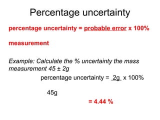
![Planning procedures
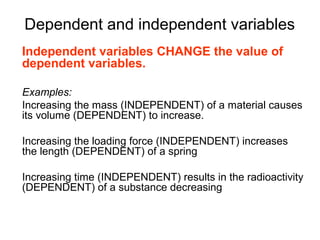
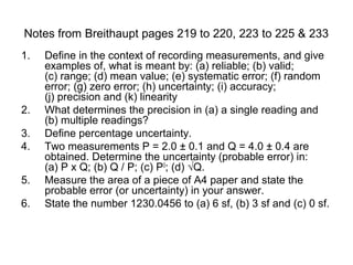
Usually the final part of a written ISA paper is a question
involving the planning of a procedure, usually related to an
ISA experiment, to test a hypothesis.
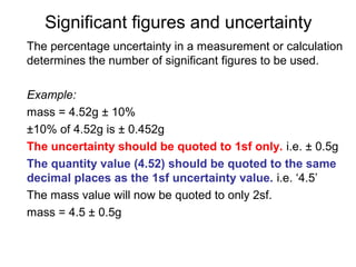
Example:
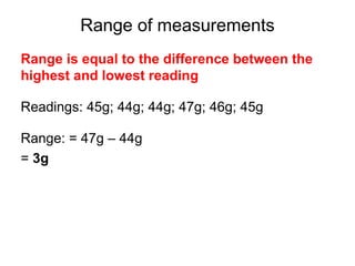
In an ISA experiment a marble was rolled down a slope.
With the slope angle kept constant the time taken by the
marble was measured for different distances down the
slope. The average speed of the marble was then measured
using the equation, speed = distance ÷ time.
Question:
Describe a procedure for measuring how the average speed
varies with slope angle. [5 marks]](https://image.slidesharecdn.com/pracerrorsas-120813093443-phpapp02/85/A2-edexcel-physics-unit-6-revision-41-320.jpg)
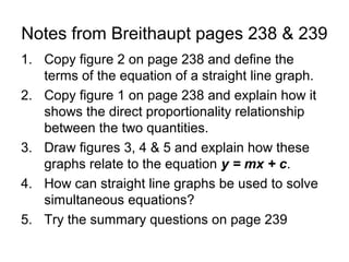

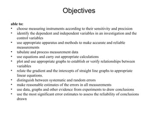
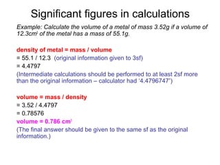
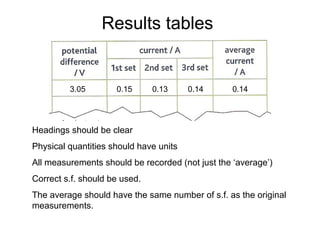
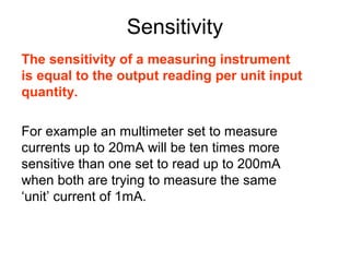
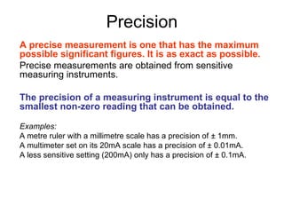
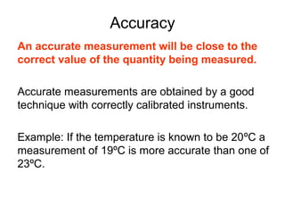
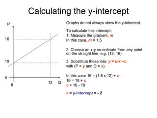
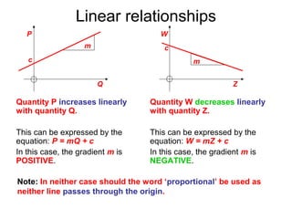
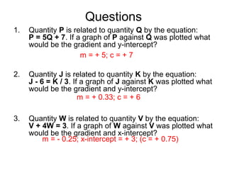
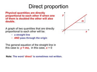
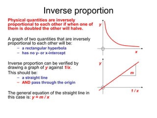
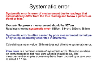
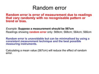
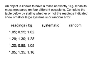
This document provides objectives and guidance for revising physics concepts related to measurement and analysis, including choosing measuring instruments, identifying variables, making measurements, processing data, using equations and graphs, identifying sources of error, and drawing valid conclusions from experimental evidence and results. Key concepts covered include significant figures, sensitivity, precision, accuracy, systematic and random error, and analyzing linear relationships through equations, direct and inverse proportion, and calculating gradients and intercepts from graphs.


![Checklist for practicals[1]](https://cdn.slidesharecdn.com/ss_thumbnails/checklistforpracticals1-110206102018-phpapp02-thumbnail.jpg?width=640&height=640&fit=bounds)


