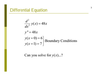
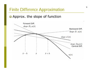
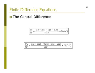
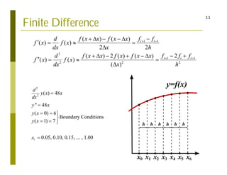
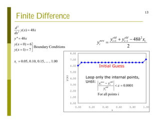
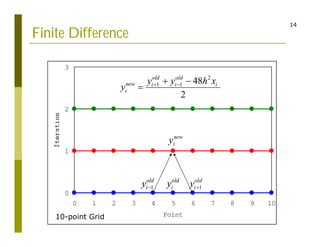
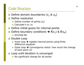
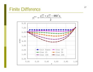
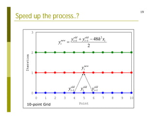
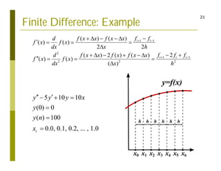
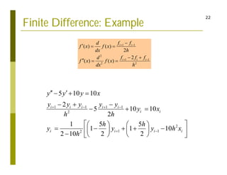
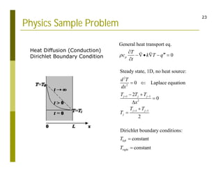
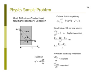
1
1
Programming, Computation, Simulation
Applications in Math & Physics
Finite Difference Methods
Syeilendra Pramuditya
Department of Physics
Institut Teknologi Bandung
2
Grid-based Computation
 Euler-type Methods
 Differential equations
 Temporal domain (variation in time)
 Initial value problems
 Initial conditions
 Finite Difference Methods
 Differential equations
 Spatial domain (variation in space)
 Boundary value problems
 Dirichlet boundary conditions: value of solution at
boundaries
 Von Neumann boundary conditions: derivative of
solution at boundaries
3
Differential Equation
2
2
( ) 48
'' 48
( 0) 6
Boundary Conditions
( 1) 7
Can you solve for ( )...?
d
y x x
dx
y x
y x
y x
y x


  

  
4
Differential Equation
3
Sure! Super easy! Just integrate twice!
( ) 8 7 6
y x x x
  
0.00
1.00
2.00
3.00
4.00
5.00
6.00
7.00
8.00
0.00 0.20 0.40 0.60 0.80 1.00
x
5
Differential Equation
2
2
( ) 5 ( ) 10 ( ) 10
5 10 10
( 0) 0
Boundary Conditions
( 1) 100
Can you solve for ( )...???
d d
y x y x y x x
dx dx
y y y x
y x
y x
y x
  
 
  
  

  
6
Derivation from Taylor Series
 Forward difference equation
7
Derivation from Taylor Series
 Backward difference equation
8
Derivation from Taylor Series
 Central difference equation
Now substract this
From this
9
Finite Difference Approximation
 Approx. the slope of function
Forward Diff.
Backward Diff.
Central Diff.
10
Finite Difference Equations
 The Central Difference
11
Finite Difference
1 1
2
1 1
2 2 2
( ) ( )
( ) ( )
2 2
2
( ) 2 ( ) ( )
( ) ( )
( )
i i
i i i
f f
d f x x f x x
f x f x
dx x h
f f f
d f x x f x f x x
f x f x
dx x h
 
 

    
   

 
     
   

2
2
( ) 48
'' 48
( 0) 6
Boundary Conditions
( 1) 7
0.05, 0.10, 0.15, ... , 1.00
i
d
y x x
dx
y x
y x
y x
x


  

  

12
Finite Difference
1 1
2
2
1 1
2
1 1
'' 48
2
48
2 48
48
2
i i i
i
i i i i
i i i
i
y x
y y y
x
h
y y y h x
y y h x
y
 
 
 

 

  
 

1 1
2
1 1
2 2
( ) ( )
2
2
( ) ( )
i i
i i i
f f
d
f x f x
dx h
f f f
d
f x f x
dx h
 
 

  
 
  
13
0.00
1.00
2.00
3.00
4.00
5.00
6.00
7.00
8.00
0.00 0.20 0.40 0.60 0.80 1.00
x
Finite Difference
Initial Guess
2
2
( ) 48
'' 48
( 0) 6
Boundary Conditions
( 1) 7
0.05, 0.10, 0.15, ... , 1.00
i
d
y x x
dx
y x
y x
y x
x


  

  

2
1 1 48
2
old old
new i i i
i
y y h x
y  
 

Loop only the internal points,
Until:
0.0001
For all points i
new old
i i
old
i
y y
y


 
14
Finite Difference
0
1
2
3
0 1 2 3 4 5 6 7 8 9 10
Point
10-point Grid
old
i
y 1
old
i
y 
1
old
i
y 
old
i
y
1
old
i
y 
new
i
y
2
1 1 48
2
old old
new i i i
i
y y h x
y  
 

15
Code Structure
 Define domain boundaries (x1 & xN)
 Define resolution
 Define number of points (xi)
 Calculate h or x
 Define initial guess for internal points
 Define boundary conditions  f(x1) & f(xN)
 Dirichlet BC
 Double Loop
 Inner loop  Update internal points using finite
difference equation
 Outer loop  Convergence check: how much the change
of each point is?
 Loop until iteration is converged
 No significant change for all points
16
Code Output
Converged in 379 iterations.
0, 6
0.05, 5.65543
0.1, 5.31675
0.15, 4.98985
0.2, 4.68064
0.25, 4.39501
0.3, 4.1389
0.35, 3.91822
0.4, 3.73892
0.45, 3.60695
0.5, 3.5283
0.55, 3.50895
0.6, 3.55492
0.65, 3.67221
0.7, 3.8669
0.75, 4.14501
0.8, 4.51263
0.85, 4.97585
0.9, 5.54074
0.95, 6.21343
1, 7
17
Finite Difference
2
1 1 48
2
old old
new i i i
i
y y h x
y  
 

0.00
1.00
2.00
3.00
4.00
5.00
6.00
7.00
8.00
0.00 0.20 0.40 0.60 0.80 1.00
x
Init Guess Iter 10
Iter 25 Iter 50
Iter 100 Iter 200
18
Finite Difference
Max error = 1E-4  379 iterations to converged
0.00
1.00
2.00
3.00
4.00
5.00
6.00
7.00
8.00
0.00 0.20 0.40 0.60 0.80 1.00
x
Exact
Finite Diff.
19
Speed up the process..?
0
1
2
3
0 1 2 3 4 5 6 7 8 9 10
Point
10-point Grid
old
i
y 1
old
i
y 
1
old
i
y 
old
i
y
1
old
i
y 
new
i
y
2
1 1 48
2
old old
new i i i
i
y y h x
y  
 

20
Speed up the process..?
2
1 1 48
2
old old
new i i i
i
y y h x
y  
 

2
1 1 48
2
old new
new i i i
i
y y h x
y  
 

Jacobi Method
Gauss-Siedel Method
379 iterations  219 iterations
1.73X Speed up!
21
Finite Difference: Example
1 1
2
1 1
2 2 2
( ) ( )
( ) ( )
2 2
2
( ) 2 ( ) ( )
( ) ( )
( )
i i
i i i
f f
d f x x f x x
f x f x
dx x h
f f f
d f x x f x f x x
f x f x
dx x h
 
 

    
  

 
     
  



5 10 10
(0) 0
( ) 100
0.0, 0.1, 0.2, ... , 1.0
i
y y y x
y
y n
x
 
  



22
Finite Difference: Example
1 1 1 1
2
2
1 1
2
5 10 10
2
5 10 10
2
1 5 5
1 1 10
2 10 2 2
i i i i i
i i
i i i i
y y y x
y y y y y
y x
h h
h h
y y y h x
h
   
 
 
  
  
  
 
   
    
   
 
    
 
1 1
2
1 1
2 2
( ) ( )
2
2
( ) ( )
i i
i i i
f f
d
f x f x
dx h
f f f
d
f x f x
dx h
 
 

  
 
  
23
Physics Sample Problem
General heat transport eq.
0
p
T
c k T q
t



   

 
2
2
1 1
2
1 1
Steady state, 1D, no heat source:
0 Laplace equation
2
0
2
Dirichlet boundary conditions:
constant
constant
j j j
j j
j
left
right
d T
dx
T T T
x
T T
T
T
T
 
 
 
 






Heat Diffusion (Conduction)
Dirichlet Boundary Condition
24
Physics Sample Problem
General heat transport eq.
0
p
T
c k T q
t



   

 
2
2
1 1
2
1 1
Steady state, 1D, no heat source:
0 Laplace equation
2
0
2
Neumann boundary conditions:
constant
constant
j j j
j j
j
left
right
d T
dx
T T T
x
T T
T
dT
dx
dT
dx
 
 
 
 






Heat Diffusion (Conduction)
Neumann Boundary Condition
Heat Flux
dT
q k
dx
  
25
Simplified Heat Conduction
 Temperature Distribution
0
10
20
30
40
50
60
70
80
90
0 1 2 3 4 5 6 7 8 9 10 11 12 13 14 15
x
T(x)
26
Code Structure
START
Set Boundary Conditions
Set Initial Guess
Repeat
Calculate interior points
Convergence check
Update interior points
Until Converge
Print Output
1 1
2
old old
new i i
i
T T
T  


for all i
new old
i i
old
i
T T
T



= for all i
old new
i i
T T
27
Physics Sample Problem
 Vibrating String
 Guitar, bass, violin, piano, etc
 Resonance frequency  standing wave with
two closed ends
28
Physics Sample Problem
 The Wave Equation
2 2
2 2
2 2
2
2 2
( , ) ( , )
Exact solution ( , ) sin( )
Guessed solution by variable separation ( , ) ( ) ( )
( ) ( )
1 1
const.
( ) ( )
m
x t x t
T
t x
x t kx t
x t y x t
d y x d t
T
y x dx t dt
 

  
 


 
 

 
  
 
   
2
2
2
2 2
2
( )
( ) Temporal domain (SHM), requires initial conditions
( )
( ) Spatial domain, requires boundary conditions
Solve the y(x) by finite difference?
d t
t
dt
d y x
y x
dx T

 
 
  
  
29
Solving Wave Equation
2 2
2
2
1 1
2
2
1 1
2 2
2
1 1
2 2
2
1 1
2 2
1 1 1 1
2 2
2
2
2
( )
( ) 0
2
0
2
0
2
2
2
2
i i i
i
i i i
i
i i
i i
i i
i
i i i i
i
d y x
y x
dx T
y y y
y
h T
y y y
y
h h T
y y
y y
h h T
y y
y
h h T
y y y y
y
h
h
T
h T
 
 
 
 
 
 
 
 
 
 
 
   
 
 
 

  

 
 

 
 
 
 
 
 


 
 
Now imagine how you would write the code..?
What are the inputs?
30
Solving Wave Equation
 Input
 String tension, T
 String length, L
 String linear density, 
 Harmonic order, n
31
Solving Wave Equation
0.0
0.5
1.0
1.5
2.0
2.5
0.0 0.2 0.4 0.6 0.8 1.0
String Length x
y(x)
Exact
Init Guess = 0.5
Init Guess = 1.0
Init Guess = 1.5

Finite Difference Method

  • 1.
    1 1 Programming, Computation, Simulation Applicationsin Math & Physics Finite Difference Methods Syeilendra Pramuditya Department of Physics Institut Teknologi Bandung
  • 2.
    2 Grid-based Computation  Euler-typeMethods  Differential equations  Temporal domain (variation in time)  Initial value problems  Initial conditions  Finite Difference Methods  Differential equations  Spatial domain (variation in space)  Boundary value problems  Dirichlet boundary conditions: value of solution at boundaries  Von Neumann boundary conditions: derivative of solution at boundaries
  • 3.
    3 Differential Equation 2 2 ( )48 '' 48 ( 0) 6 Boundary Conditions ( 1) 7 Can you solve for ( )...? d y x x dx y x y x y x y x         
  • 4.
    4 Differential Equation 3 Sure! Supereasy! Just integrate twice! ( ) 8 7 6 y x x x    0.00 1.00 2.00 3.00 4.00 5.00 6.00 7.00 8.00 0.00 0.20 0.40 0.60 0.80 1.00 x
  • 5.
    5 Differential Equation 2 2 ( )5 ( ) 10 ( ) 10 5 10 10 ( 0) 0 Boundary Conditions ( 1) 100 Can you solve for ( )...??? d d y x y x y x x dx dx y y y x y x y x y x               
  • 6.
    6 Derivation from TaylorSeries  Forward difference equation
  • 7.
    7 Derivation from TaylorSeries  Backward difference equation
  • 8.
    8 Derivation from TaylorSeries  Central difference equation Now substract this From this
  • 9.
    9 Finite Difference Approximation Approx. the slope of function Forward Diff. Backward Diff. Central Diff.
  • 10.
    10 Finite Difference Equations The Central Difference
  • 11.
    11 Finite Difference 1 1 2 11 2 2 2 ( ) ( ) ( ) ( ) 2 2 2 ( ) 2 ( ) ( ) ( ) ( ) ( ) i i i i i f f d f x x f x x f x f x dx x h f f f d f x x f x f x x f x f x dx x h                             2 2 ( ) 48 '' 48 ( 0) 6 Boundary Conditions ( 1) 7 0.05, 0.10, 0.15, ... , 1.00 i d y x x dx y x y x y x x          
  • 12.
    12 Finite Difference 1 1 2 2 11 2 1 1 '' 48 2 48 2 48 48 2 i i i i i i i i i i i i y x y y y x h y y y h x y y h x y                 1 1 2 1 1 2 2 ( ) ( ) 2 2 ( ) ( ) i i i i i f f d f x f x dx h f f f d f x f x dx h             
  • 13.
    13 0.00 1.00 2.00 3.00 4.00 5.00 6.00 7.00 8.00 0.00 0.20 0.400.60 0.80 1.00 x Finite Difference Initial Guess 2 2 ( ) 48 '' 48 ( 0) 6 Boundary Conditions ( 1) 7 0.05, 0.10, 0.15, ... , 1.00 i d y x x dx y x y x y x x           2 1 1 48 2 old old new i i i i y y h x y      Loop only the internal points, Until: 0.0001 For all points i new old i i old i y y y    
  • 14.
    14 Finite Difference 0 1 2 3 0 12 3 4 5 6 7 8 9 10 Point 10-point Grid old i y 1 old i y  1 old i y  old i y 1 old i y  new i y 2 1 1 48 2 old old new i i i i y y h x y     
  • 15.
    15 Code Structure  Definedomain boundaries (x1 & xN)  Define resolution  Define number of points (xi)  Calculate h or x  Define initial guess for internal points  Define boundary conditions  f(x1) & f(xN)  Dirichlet BC  Double Loop  Inner loop  Update internal points using finite difference equation  Outer loop  Convergence check: how much the change of each point is?  Loop until iteration is converged  No significant change for all points
  • 16.
    16 Code Output Converged in379 iterations. 0, 6 0.05, 5.65543 0.1, 5.31675 0.15, 4.98985 0.2, 4.68064 0.25, 4.39501 0.3, 4.1389 0.35, 3.91822 0.4, 3.73892 0.45, 3.60695 0.5, 3.5283 0.55, 3.50895 0.6, 3.55492 0.65, 3.67221 0.7, 3.8669 0.75, 4.14501 0.8, 4.51263 0.85, 4.97585 0.9, 5.54074 0.95, 6.21343 1, 7
  • 17.
    17 Finite Difference 2 1 148 2 old old new i i i i y y h x y      0.00 1.00 2.00 3.00 4.00 5.00 6.00 7.00 8.00 0.00 0.20 0.40 0.60 0.80 1.00 x Init Guess Iter 10 Iter 25 Iter 50 Iter 100 Iter 200
  • 18.
    18 Finite Difference Max error= 1E-4  379 iterations to converged 0.00 1.00 2.00 3.00 4.00 5.00 6.00 7.00 8.00 0.00 0.20 0.40 0.60 0.80 1.00 x Exact Finite Diff.
  • 19.
    19 Speed up theprocess..? 0 1 2 3 0 1 2 3 4 5 6 7 8 9 10 Point 10-point Grid old i y 1 old i y  1 old i y  old i y 1 old i y  new i y 2 1 1 48 2 old old new i i i i y y h x y     
  • 20.
    20 Speed up theprocess..? 2 1 1 48 2 old old new i i i i y y h x y      2 1 1 48 2 old new new i i i i y y h x y      Jacobi Method Gauss-Siedel Method 379 iterations  219 iterations 1.73X Speed up!
  • 21.
    21 Finite Difference: Example 11 2 1 1 2 2 2 ( ) ( ) ( ) ( ) 2 2 2 ( ) 2 ( ) ( ) ( ) ( ) ( ) i i i i i f f d f x x f x x f x f x dx x h f f f d f x x f x f x x f x f x dx x h                             5 10 10 (0) 0 ( ) 100 0.0, 0.1, 0.2, ... , 1.0 i y y y x y y n x        
  • 22.
    22 Finite Difference: Example 11 1 1 2 2 1 1 2 5 10 10 2 5 10 10 2 1 5 5 1 1 10 2 10 2 2 i i i i i i i i i i i y y y x y y y y y y x h h h h y y y h x h                                          1 1 2 1 1 2 2 ( ) ( ) 2 2 ( ) ( ) i i i i i f f d f x f x dx h f f f d f x f x dx h             
  • 23.
    23 Physics Sample Problem Generalheat transport eq. 0 p T c k T q t           2 2 1 1 2 1 1 Steady state, 1D, no heat source: 0 Laplace equation 2 0 2 Dirichlet boundary conditions: constant constant j j j j j j left right d T dx T T T x T T T T T               Heat Diffusion (Conduction) Dirichlet Boundary Condition
  • 24.
    24 Physics Sample Problem Generalheat transport eq. 0 p T c k T q t           2 2 1 1 2 1 1 Steady state, 1D, no heat source: 0 Laplace equation 2 0 2 Neumann boundary conditions: constant constant j j j j j j left right d T dx T T T x T T T dT dx dT dx               Heat Diffusion (Conduction) Neumann Boundary Condition Heat Flux dT q k dx   
  • 25.
    25 Simplified Heat Conduction Temperature Distribution 0 10 20 30 40 50 60 70 80 90 0 1 2 3 4 5 6 7 8 9 10 11 12 13 14 15 x T(x)
  • 26.
    26 Code Structure START Set BoundaryConditions Set Initial Guess Repeat Calculate interior points Convergence check Update interior points Until Converge Print Output 1 1 2 old old new i i i T T T     for all i new old i i old i T T T    = for all i old new i i T T
  • 27.
    27 Physics Sample Problem Vibrating String  Guitar, bass, violin, piano, etc  Resonance frequency  standing wave with two closed ends
  • 28.
    28 Physics Sample Problem The Wave Equation 2 2 2 2 2 2 2 2 2 ( , ) ( , ) Exact solution ( , ) sin( ) Guessed solution by variable separation ( , ) ( ) ( ) ( ) ( ) 1 1 const. ( ) ( ) m x t x t T t x x t kx t x t y x t d y x d t T y x dx t dt                           2 2 2 2 2 2 ( ) ( ) Temporal domain (SHM), requires initial conditions ( ) ( ) Spatial domain, requires boundary conditions Solve the y(x) by finite difference? d t t dt d y x y x dx T           
  • 29.
    29 Solving Wave Equation 22 2 2 1 1 2 2 1 1 2 2 2 1 1 2 2 2 1 1 2 2 1 1 1 1 2 2 2 2 2 ( ) ( ) 0 2 0 2 0 2 2 2 2 i i i i i i i i i i i i i i i i i i i i d y x y x dx T y y y y h T y y y y h h T y y y y h h T y y y h h T y y y y y h h T h T                                                             Now imagine how you would write the code..? What are the inputs?
  • 30.
    30 Solving Wave Equation Input  String tension, T  String length, L  String linear density,   Harmonic order, n
  • 31.
    31 Solving Wave Equation 0.0 0.5 1.0 1.5 2.0 2.5 0.00.2 0.4 0.6 0.8 1.0 String Length x y(x) Exact Init Guess = 0.5 Init Guess = 1.0 Init Guess = 1.5