The document provides information about the normal distribution and standard normal distribution:
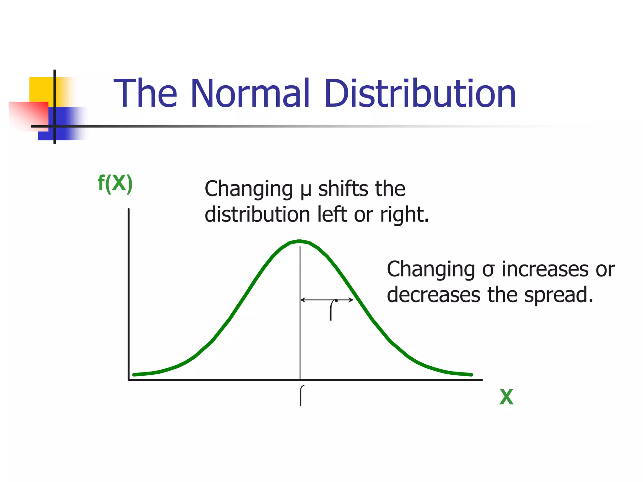
- The normal distribution is defined by its mean (μ) and standard deviation (σ). Changing μ shifts the distribution left or right, while changing σ increases or decreases the spread.
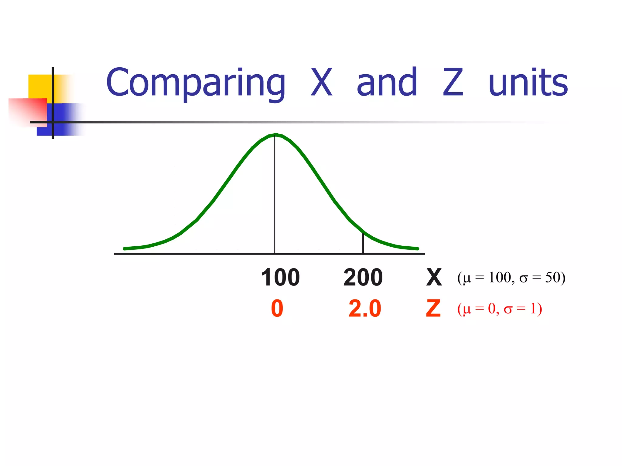
- All normal distributions can be converted to the standard normal distribution (with μ=0 and σ=1) by subtracting the mean and dividing by the standard deviation.
- The standard normal distribution is useful because probability tables and computer programs provide the integral values, avoiding the need to calculate integrals manually.
- For a normal distribution, approximately 68% of the data falls within 1 standard deviation of the mean, 95% falls
Explores the normal distribution, including definitions, shifts, and spreads based on mean (μ) and standard deviation (σ). Key concept: bell curve.
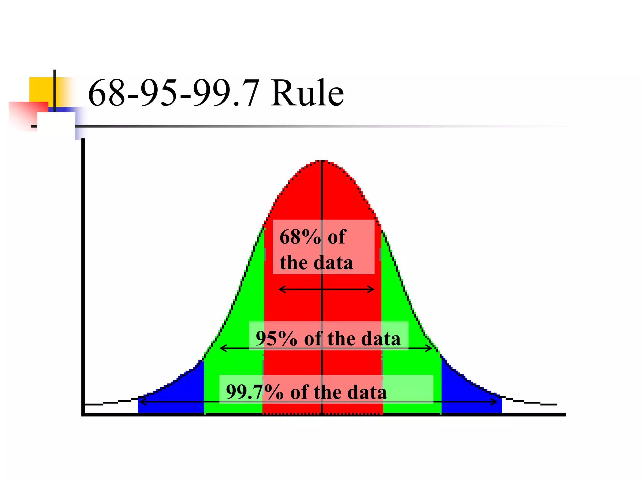
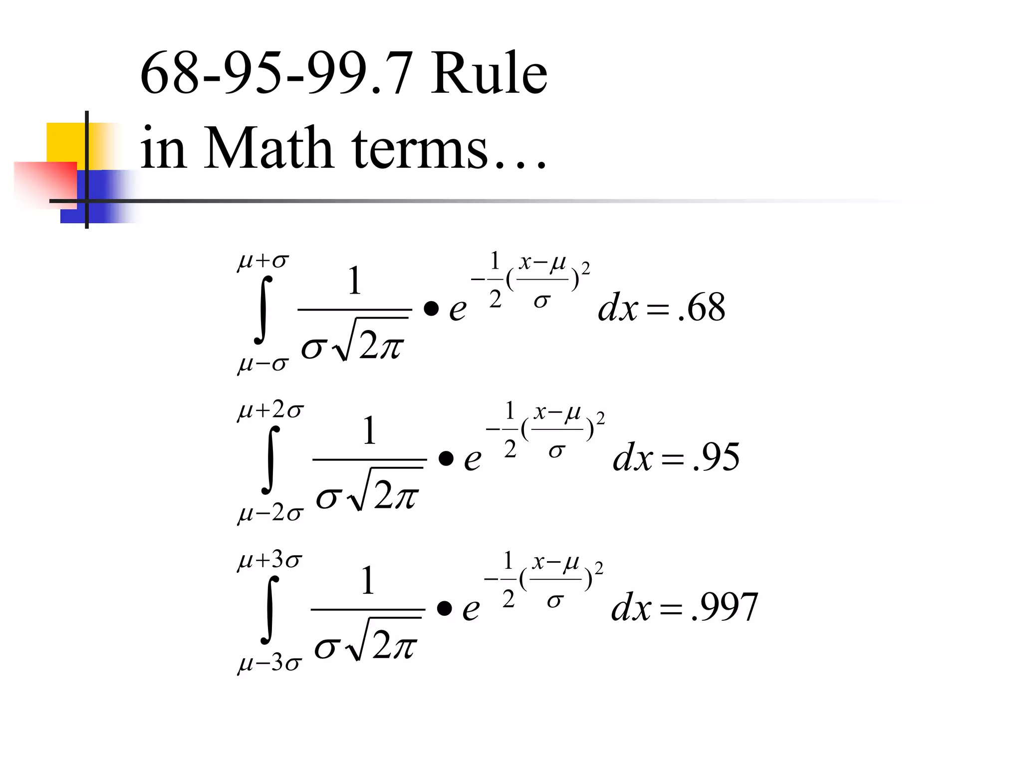
Highlights the 68-95-99.7 rule, indicating percentages of data that fall within 1, 2, and 3 standard deviations of the mean.
Demonstrates the application of normal distribution through examples in runner's weights and explanations of how many fall within standard deviations.
Uses SAT scores to illustrate how normal distribution operates, detailing score ranges for various percentiles.
Introduces the standard normal distribution (Z), including conversion samples, probability calculations, and examples using birth weights.
Discusses methods to evaluate if data is normally distributed through histograms, summary measures, and probability plots.
Presents examples of class data measures (mean, median, mode) and ranges, focusing on normal distribution properties in practice.
Explains normal probability plots, evaluates skewness in datasets, and discusses testing for normality with formal tests.Details the conditions under which binomial distributions can be approximated by normal distributions, including examples and calculations.
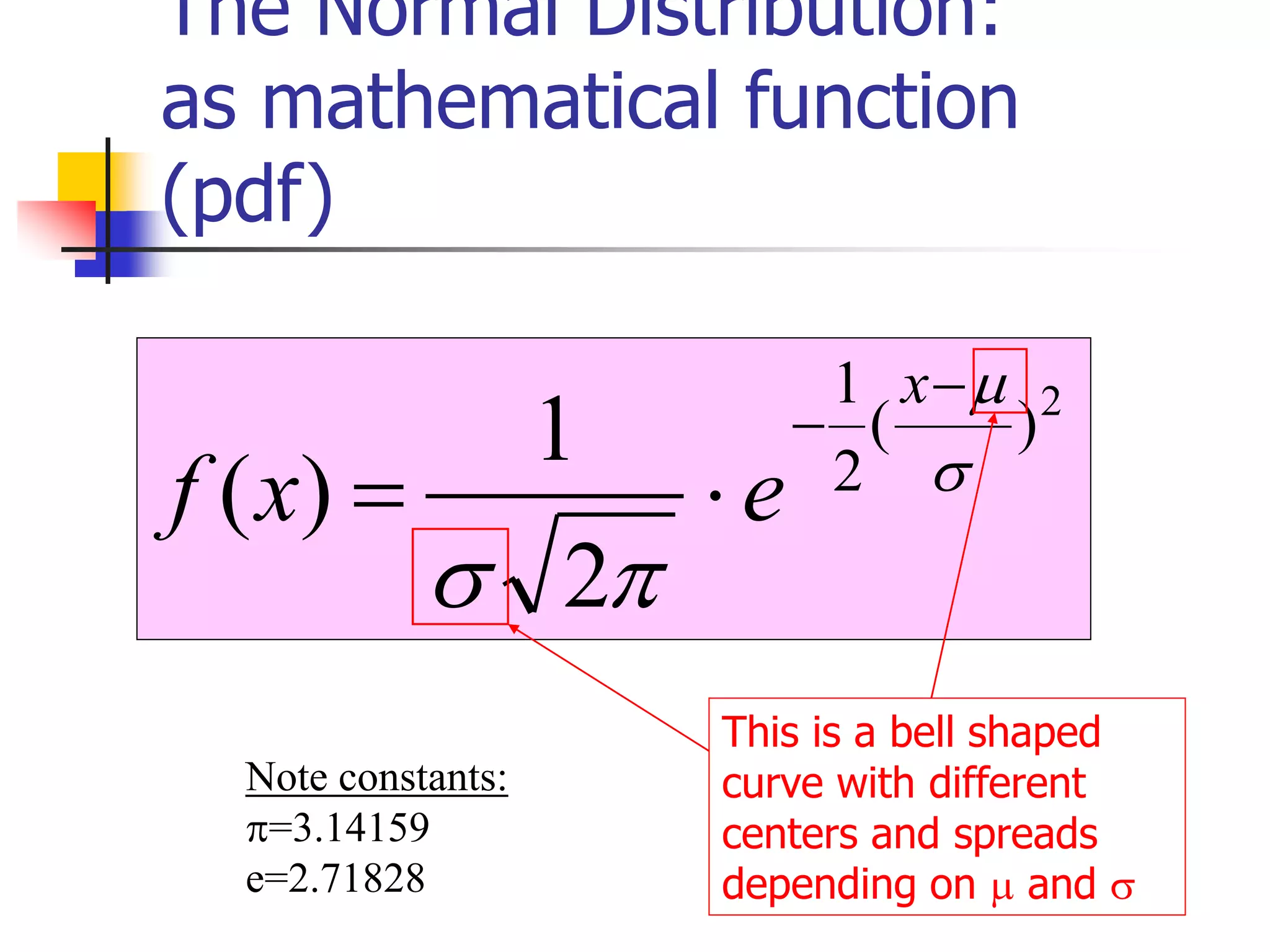
The Normal Distribution:
asmathematical function
(pdf)
2
)
(
2
1
2
1
)
(
x
e
x
f
Note constants:
=3.14159
e=2.71828
This is a bell shaped
curve with different
centers and spreads
depending on and
4.
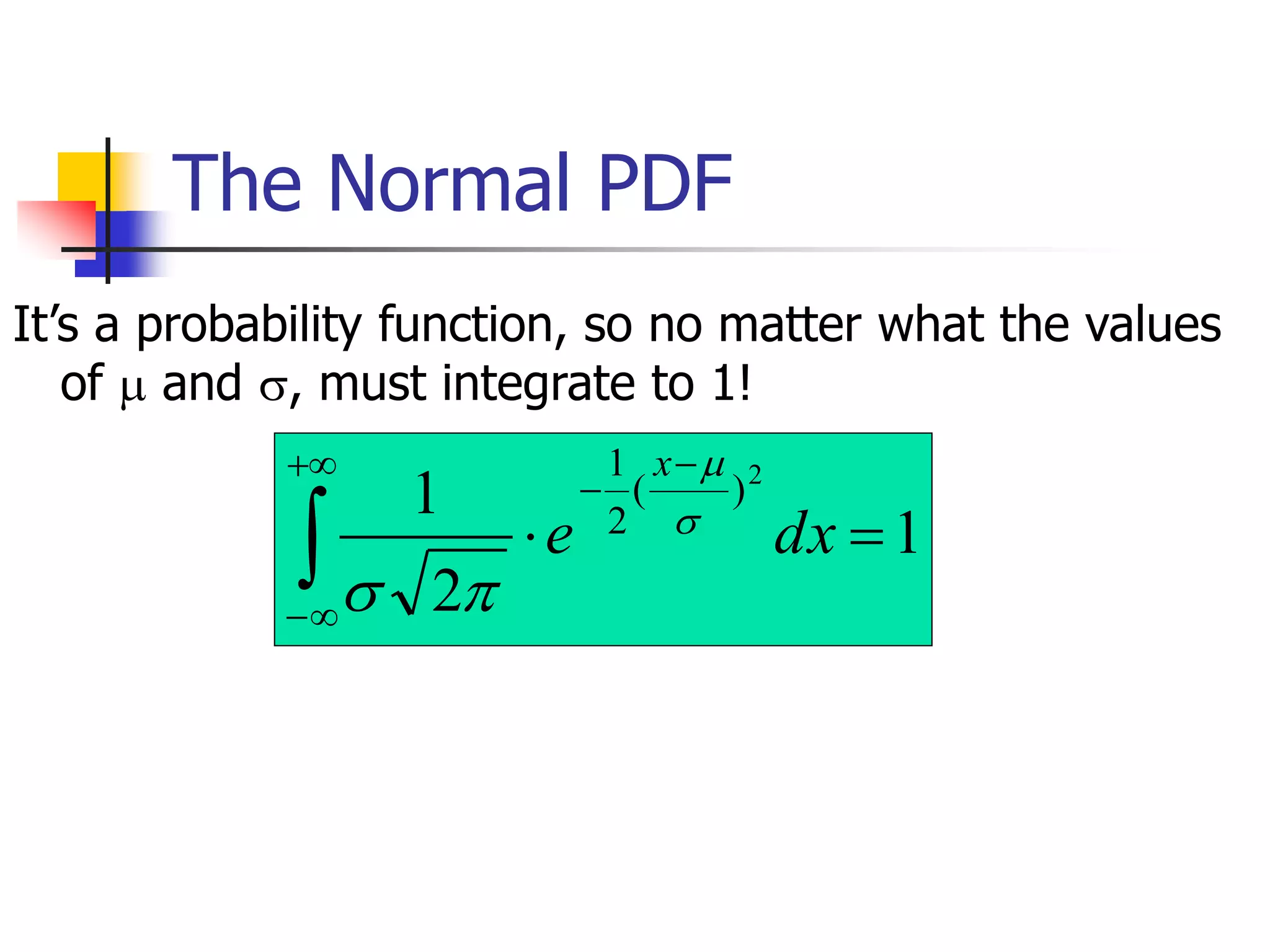
The Normal PDF
1
2
12
)
(
2
1
dx
e
x
It’s a probability function, so no matter what the values
of and , must integrate to 1!
5.
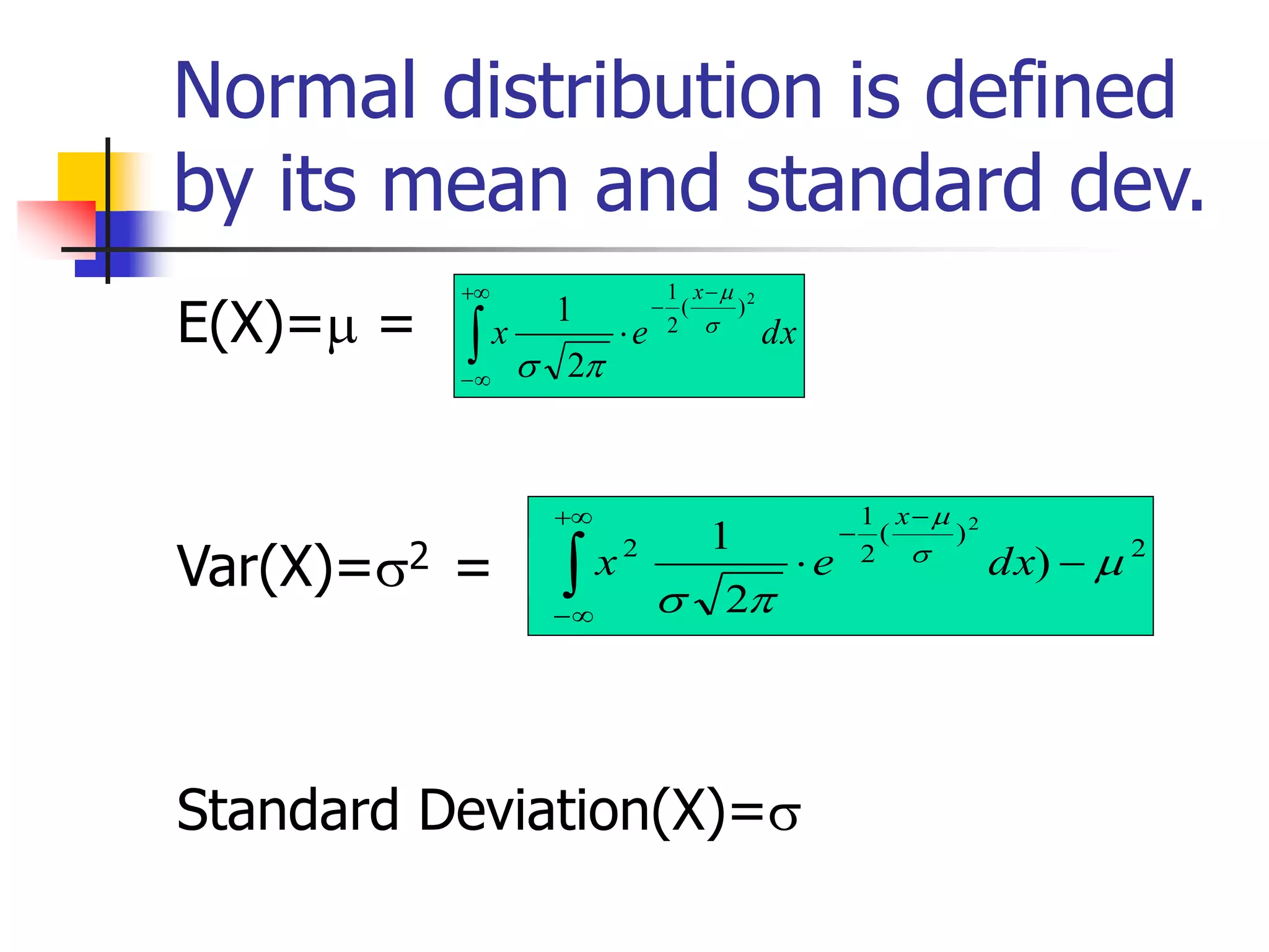
Normal distribution isdefined
by its mean and standard dev.
E(X)= =
Var(X)=2 =
Standard Deviation(X)=
dx
e
x
x
2
)
(
2
1
2
1
2
)
(
2
1
2
)
2
1
(
2
dx
e
x
x
6.
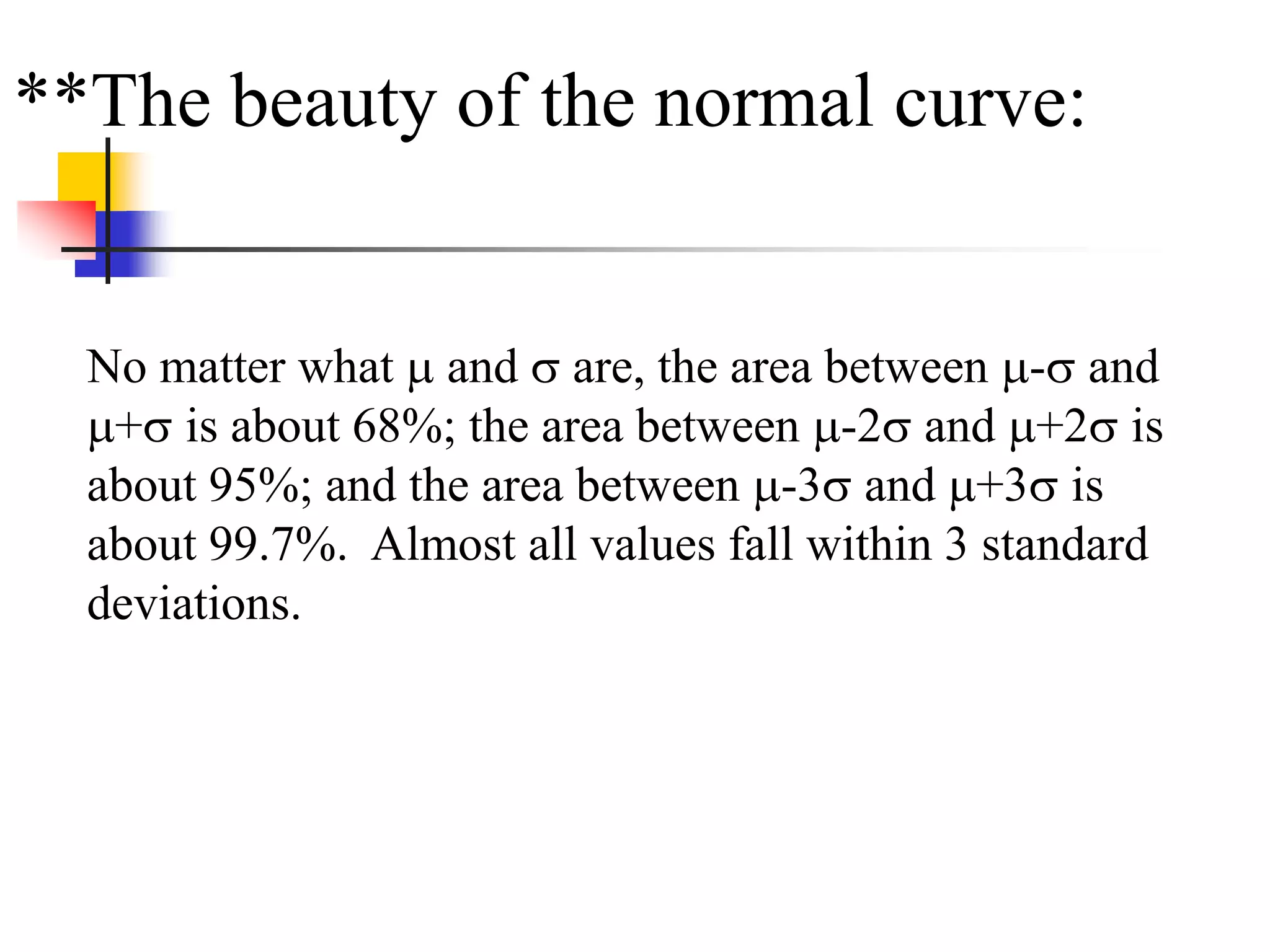
**The beauty ofthe normal curve:
No matter what and are, the area between - and
+ is about 68%; the area between -2 and +2 is
about 95%; and the area between -3 and +3 is
about 99.7%. Almost all values fall within 3 standard
deviations.
How good isrule for real data?
Check some example data:
The mean of the weight of the women = 127.8
The standard deviation (SD) = 15.5
10.
8 0 90 1 0 0 1 1 0 1 2 0 1 3 0 1 4 0 1 5 0 1 6 0
0
5
1 0
1 5
2 0
2 5
P
e
r
c
e
n
t
P O U N D S
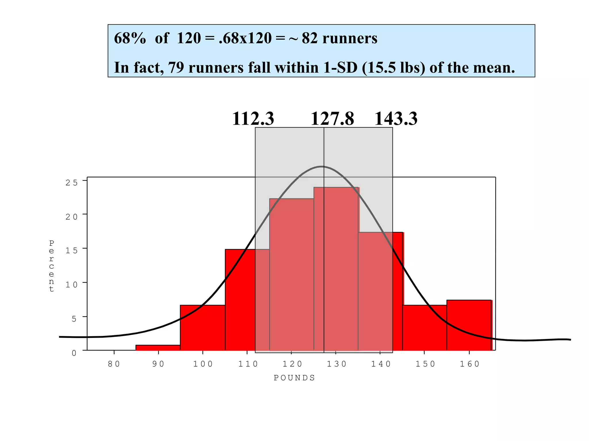
127.8 143.3
112.3
68% of 120 = .68x120 = ~ 82 runners
In fact, 79 runners fall within 1-SD (15.5 lbs) of the mean.
11.
8 0 90 1 0 0 1 1 0 1 2 0 1 3 0 1 4 0 1 5 0 1 6 0
0
5
1 0
1 5
2 0
2 5
P
e
r
c
e
n
t
P O U N D S
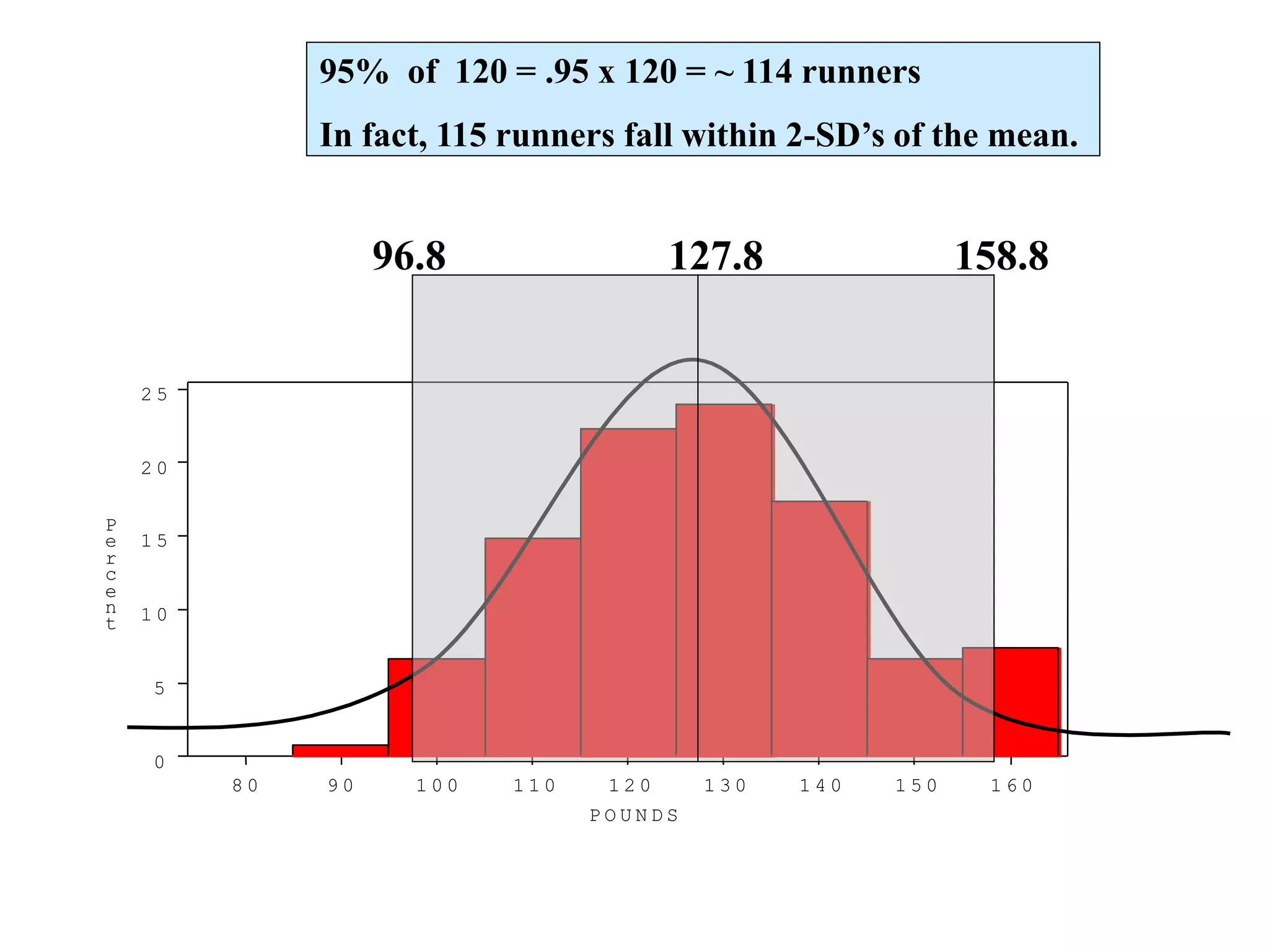
127.8
96.8
95% of 120 = .95 x 120 = ~ 114 runners
In fact, 115 runners fall within 2-SD’s of the mean.
158.8
12.
8 0 90 1 0 0 1 1 0 1 2 0 1 3 0 1 4 0 1 5 0 1 6 0
0
5
1 0
1 5
2 0
2 5
P
e
r
c
e
n
t
P O U N D S
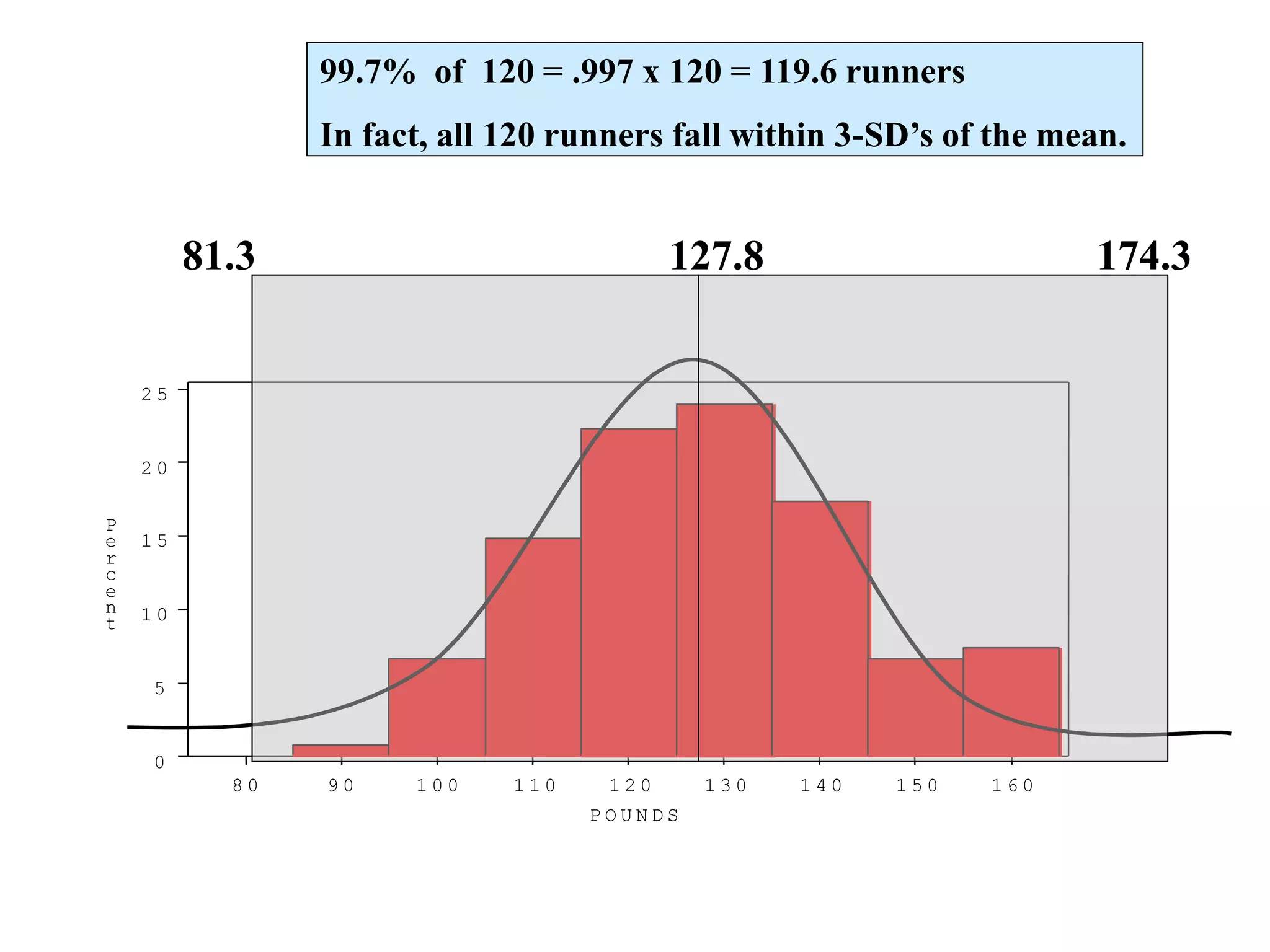
127.8
81.3
99.7% of 120 = .997 x 120 = 119.6 runners
In fact, all 120 runners fall within 3-SD’s of the mean.
174.3
13.
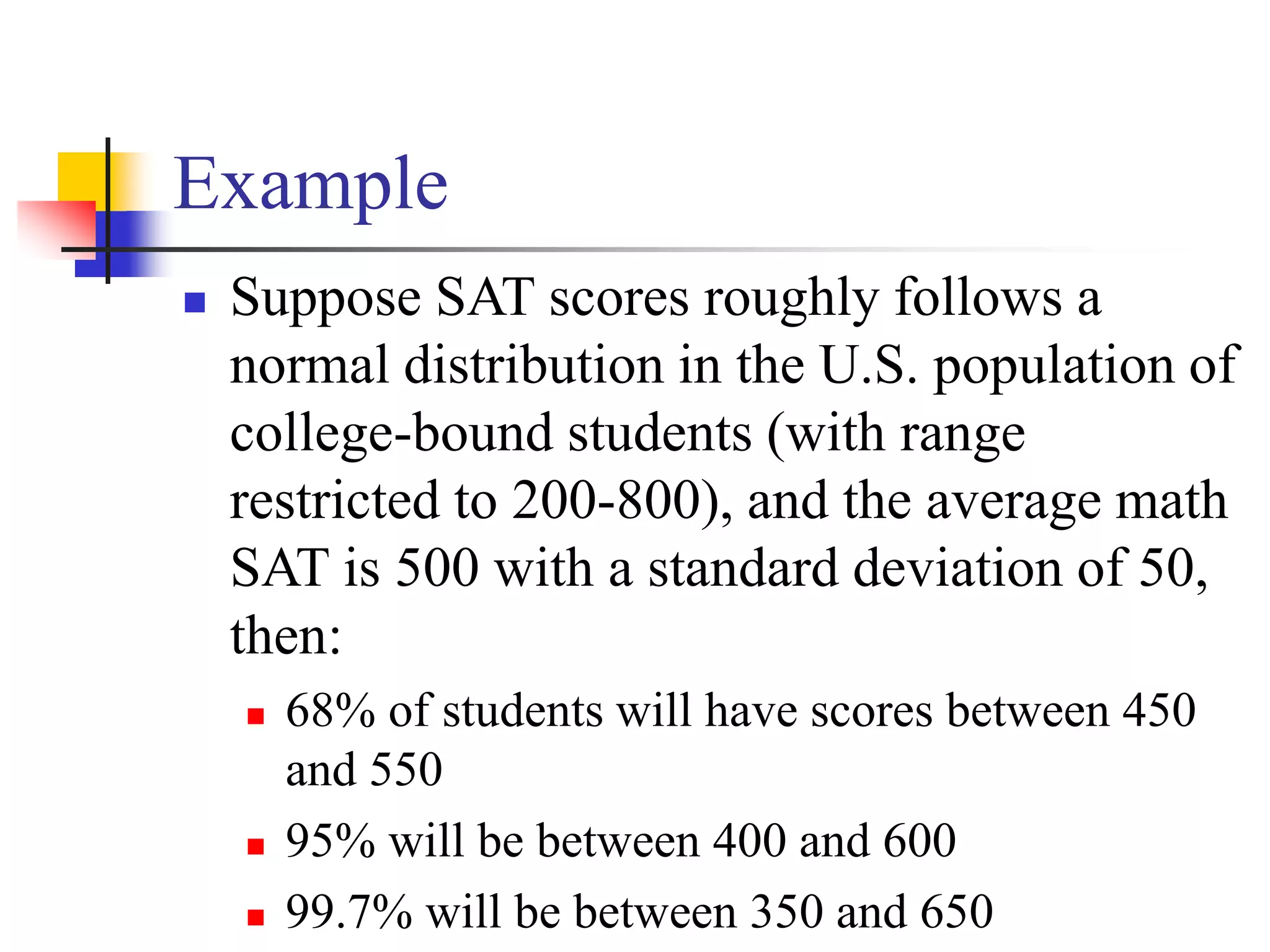
Example
Suppose SATscores roughly follows a
normal distribution in the U.S. population of
college-bound students (with range
restricted to 200-800), and the average math
SAT is 500 with a standard deviation of 50,
then:
68% of students will have scores between 450
and 550
95% will be between 400 and 600
99.7% will be between 350 and 650
14.
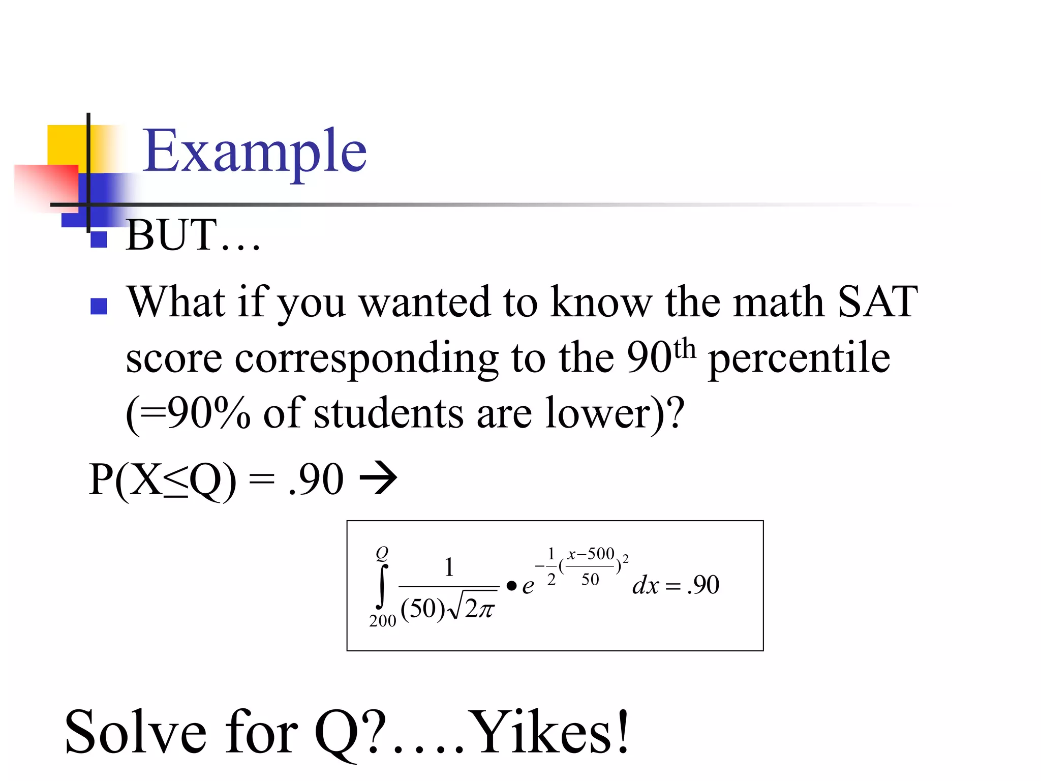
Example
BUT…
Whatif you wanted to know the math SAT
score corresponding to the 90th percentile
(=90% of students are lower)?
P(X≤Q) = .90
90
.
2
)
50
(
1
200
)
50
500
(
2
1 2
Q x
dx
e
Solve for Q?….Yikes!
15.
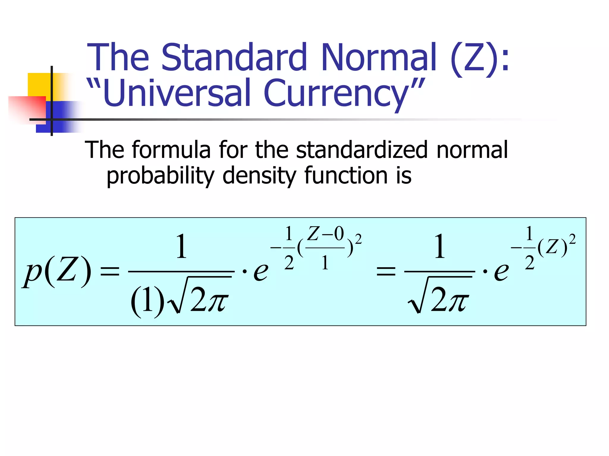
The Standard Normal(Z):
“Universal Currency”
The formula for the standardized normal
probability density function is
2
2
)
(
2
1
)
1
0
(
2
1
2
1
2
)
1
(
1
)
(
Z
Z
e
e
Z
p
16.
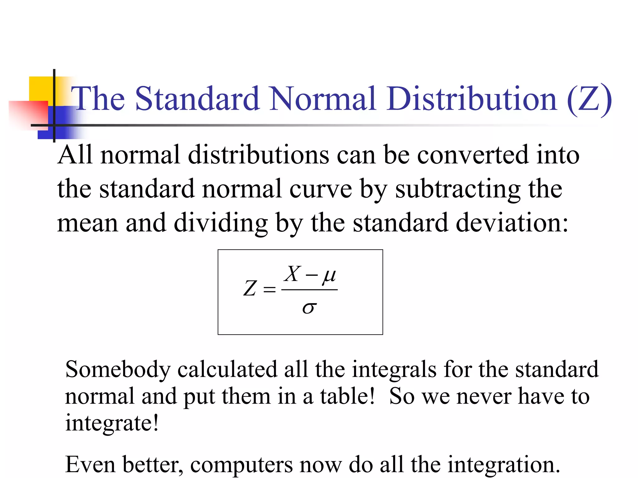
The Standard NormalDistribution (Z)
All normal distributions can be converted into
the standard normal curve by subtracting the
mean and dividing by the standard deviation:
X
Z
Somebody calculated all the integrals for the standard
normal and put them in a table! So we never have to
integrate!
Even better, computers now do all the integration.
17.
Comparing X andZ units
Z
100
2.0
0
200 X ( = 100, = 50)
( = 0, = 1)
18.
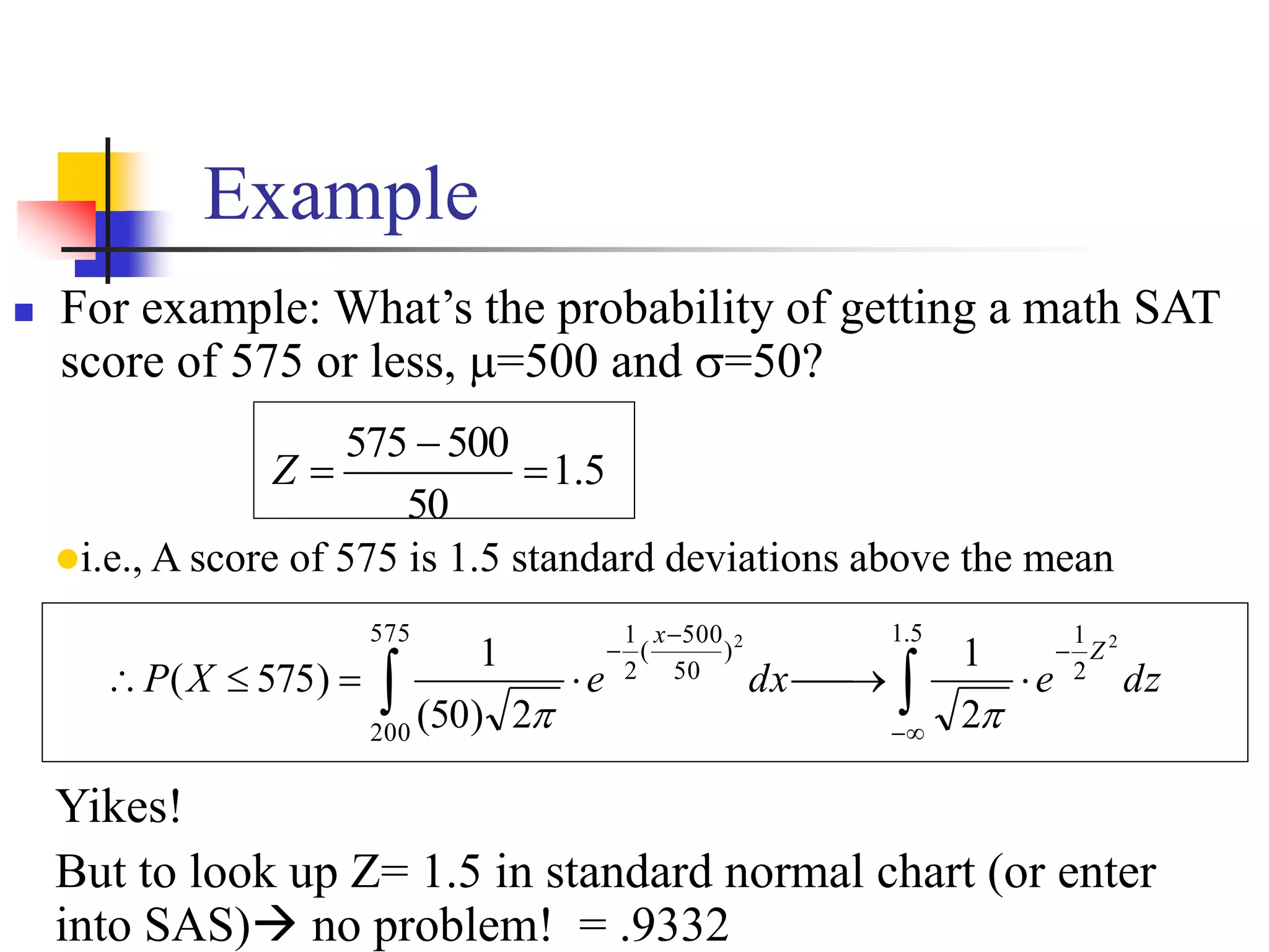
Example
For example:What’s the probability of getting a math SAT
score of 575 or less, =500 and =50?
5
.
1
50
500
575
Z
i.e., A score of 575 is 1.5 standard deviations above the mean
5
.
1
2
1
575
200
)
50
500
(
2
1 2
2
2
1
2
)
50
(
1
)
575
( dz
e
dx
e
X
P
Z
x
Yikes!
But to look up Z= 1.5 in standard normal chart (or enter
into SAS) no problem! = .9332
19.
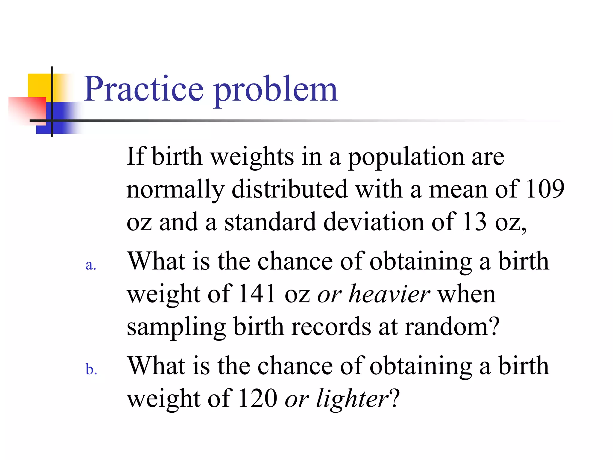
Practice problem
If birthweights in a population are
normally distributed with a mean of 109
oz and a standard deviation of 13 oz,
a. What is the chance of obtaining a birth
weight of 141 oz or heavier when
sampling birth records at random?
b. What is the chance of obtaining a birth
weight of 120 or lighter?
20.
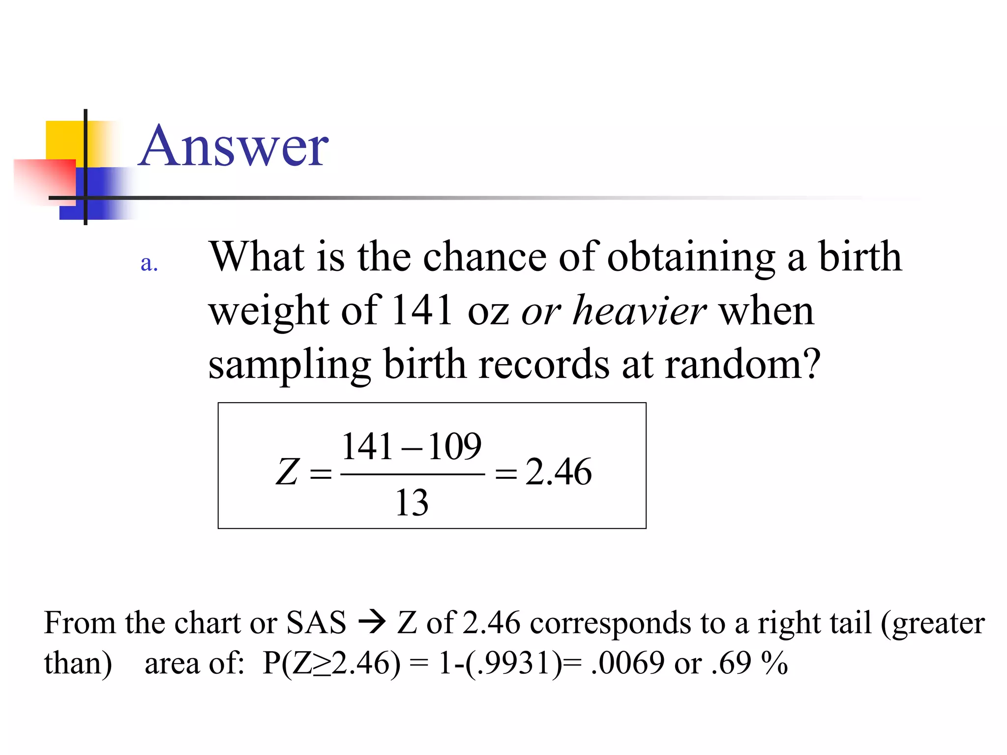
Answer
a. What isthe chance of obtaining a birth
weight of 141 oz or heavier when
sampling birth records at random?
46
.
2
13
109
141
Z
From the chart or SAS Z of 2.46 corresponds to a right tail (greater
than) area of: P(Z≥2.46) = 1-(.9931)= .0069 or .69 %
21.
Answer
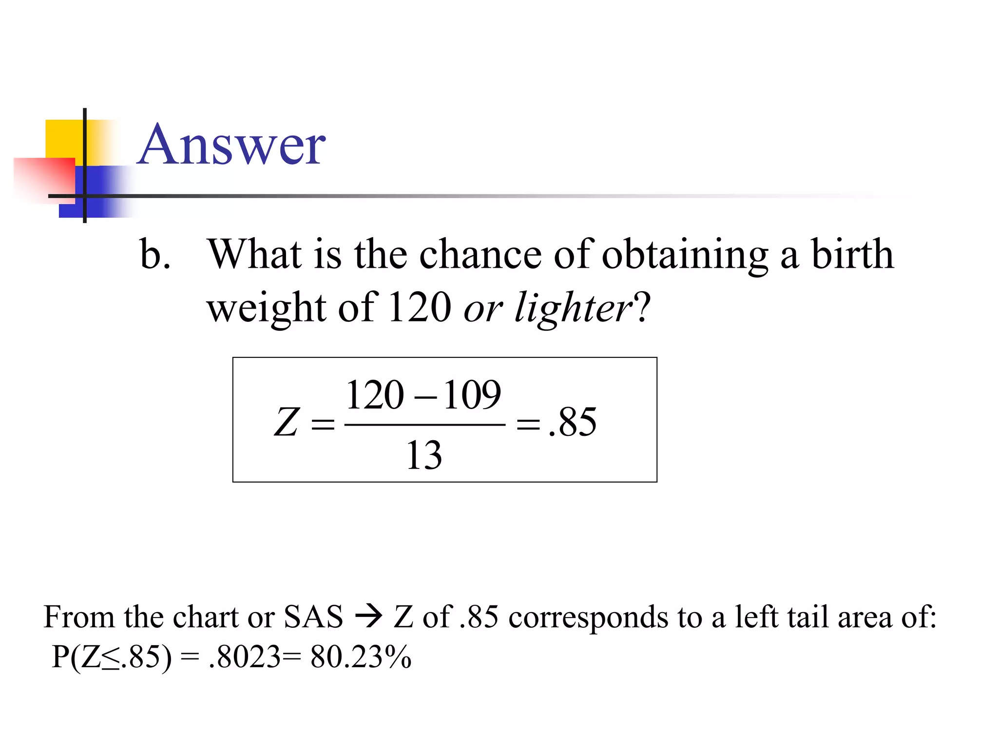
b. What isthe chance of obtaining a birth
weight of 120 or lighter?
From the chart or SAS Z of .85 corresponds to a left tail area of:
P(Z≤.85) = .8023= 80.23%
85
.
13
109
120
Z
22.
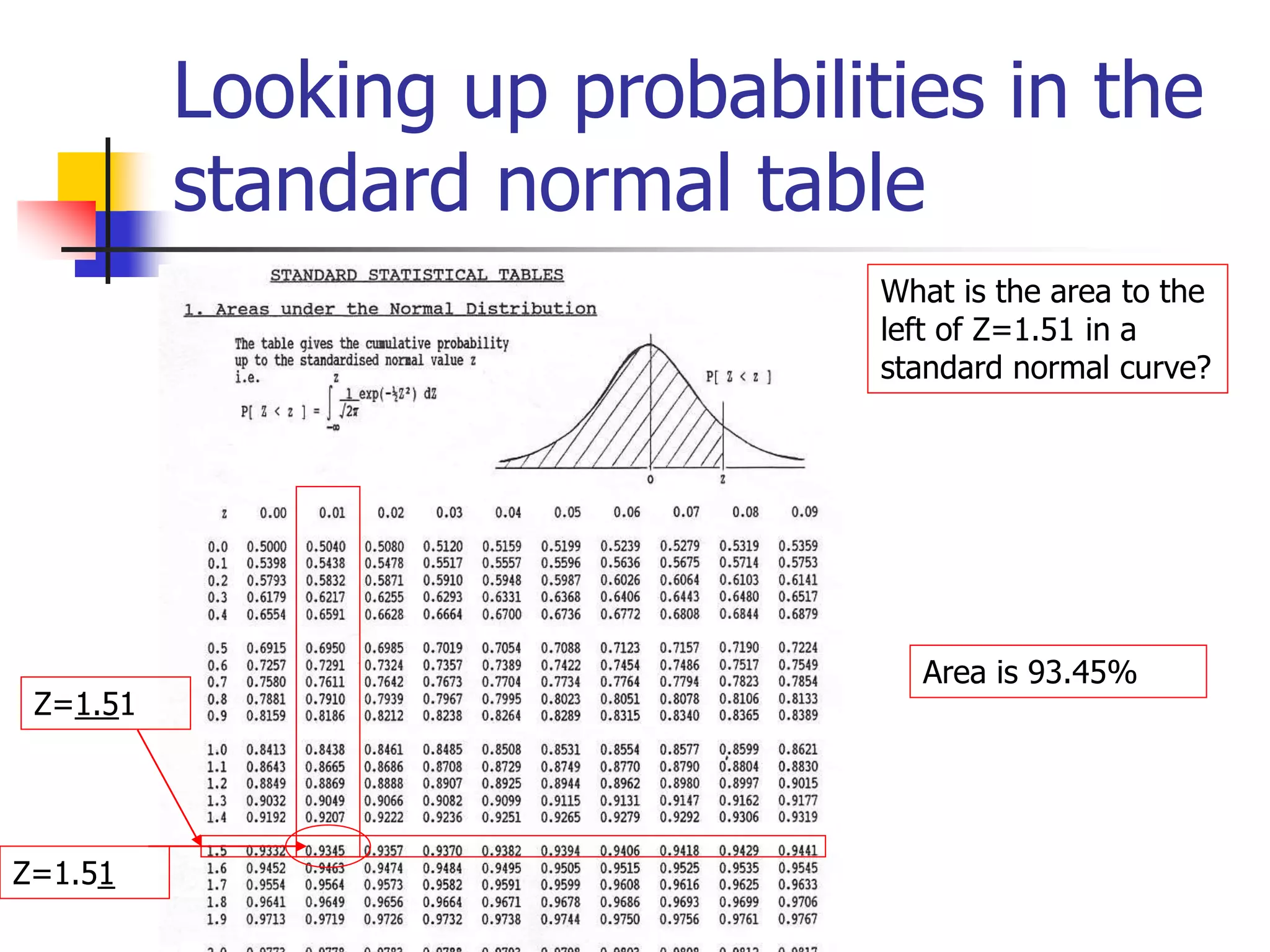
Looking up probabilitiesin the
standard normal table
What is the area to the
left of Z=1.51 in a
standard normal curve?
Z=1.51
Z=1.51
Area is 93.45%
23.
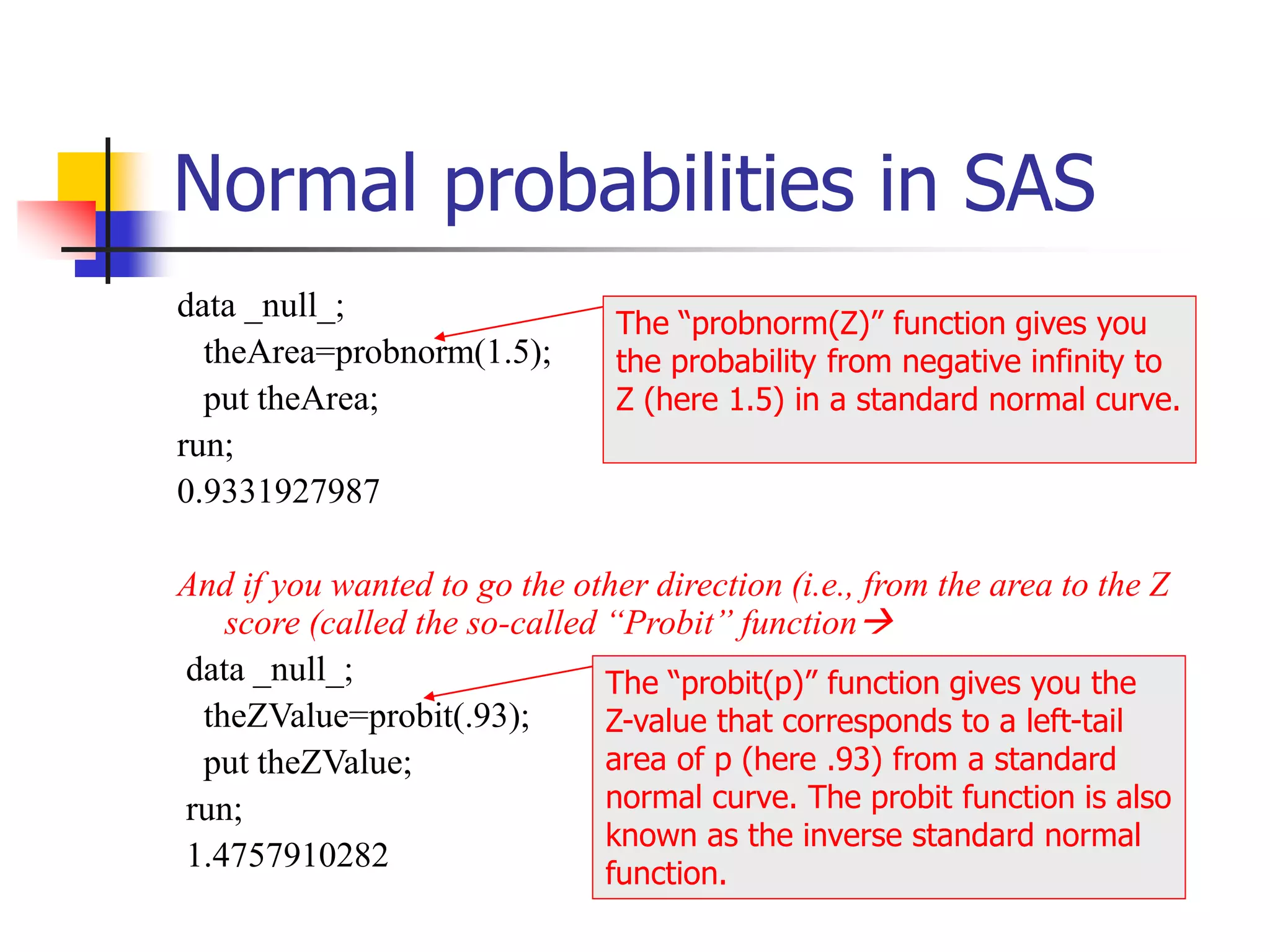
Normal probabilities inSAS
data _null_;
theArea=probnorm(1.5);
put theArea;
run;
0.9331927987
And if you wanted to go the other direction (i.e., from the area to the Z
score (called the so-called “Probit” function
data _null_;
theZValue=probit(.93);
put theZValue;
run;
1.4757910282
The “probnorm(Z)” function gives you
the probability from negative infinity to
Z (here 1.5) in a standard normal curve.
The “probit(p)” function gives you the
Z-value that corresponds to a left-tail
area of p (here .93) from a standard
normal curve. The probit function is also
known as the inverse standard normal
function.
24.
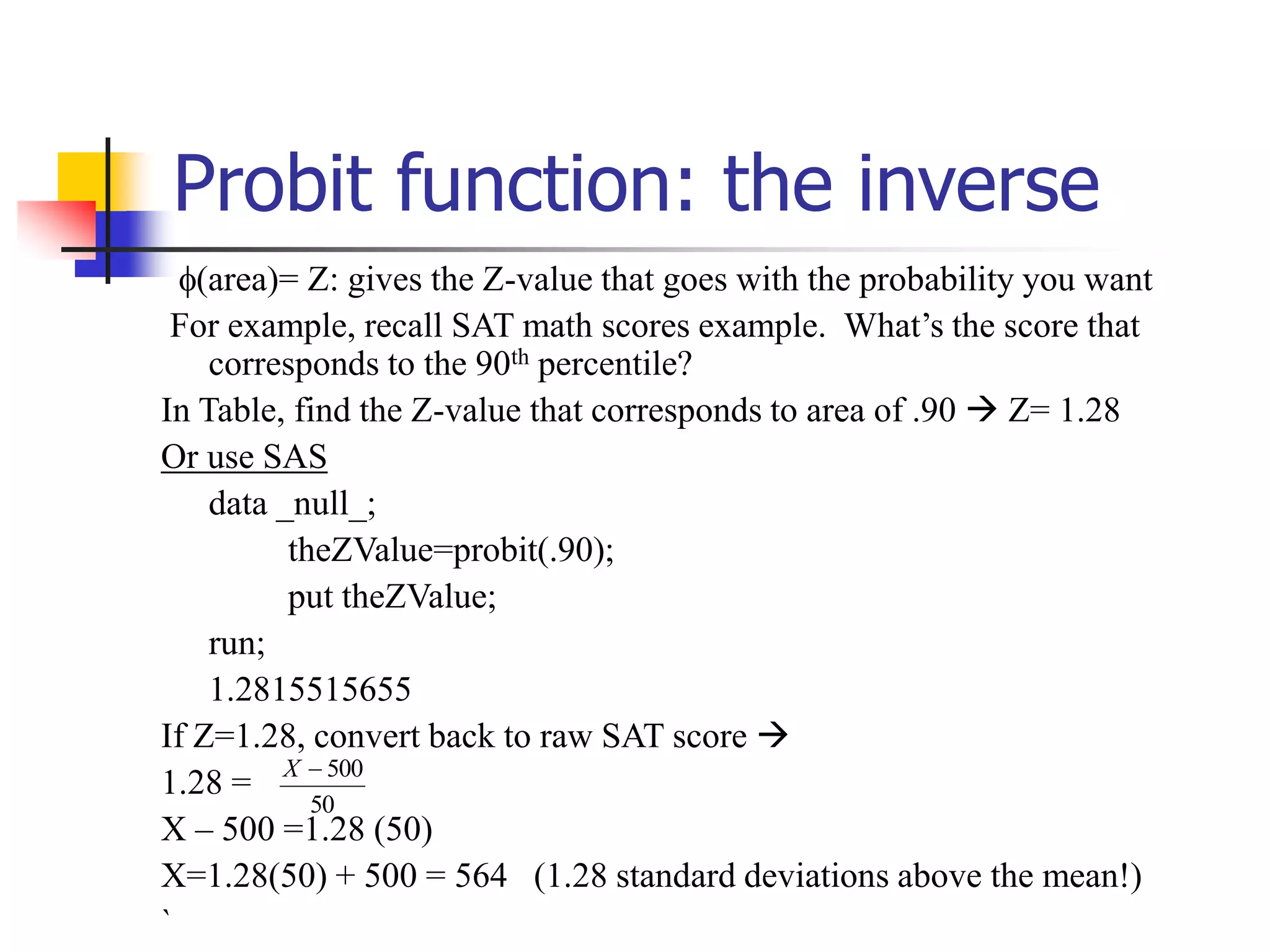
Probit function: theinverse
(area)= Z: gives the Z-value that goes with the probability you want
For example, recall SAT math scores example. What’s the score that
corresponds to the 90th percentile?
In Table, find the Z-value that corresponds to area of .90 Z= 1.28
Or use SAS
data _null_;
theZValue=probit(.90);
put theZValue;
run;
1.2815515655
If Z=1.28, convert back to raw SAT score
1.28 =
X – 500 =1.28 (50)
X=1.28(50) + 500 = 564 (1.28 standard deviations above the mean!)
`
50
500
X
25.
Are my data“normal”?
Not all continuous random variables are
normally distributed!!
It is important to evaluate how well the
data are approximated by a normal
distribution
26.
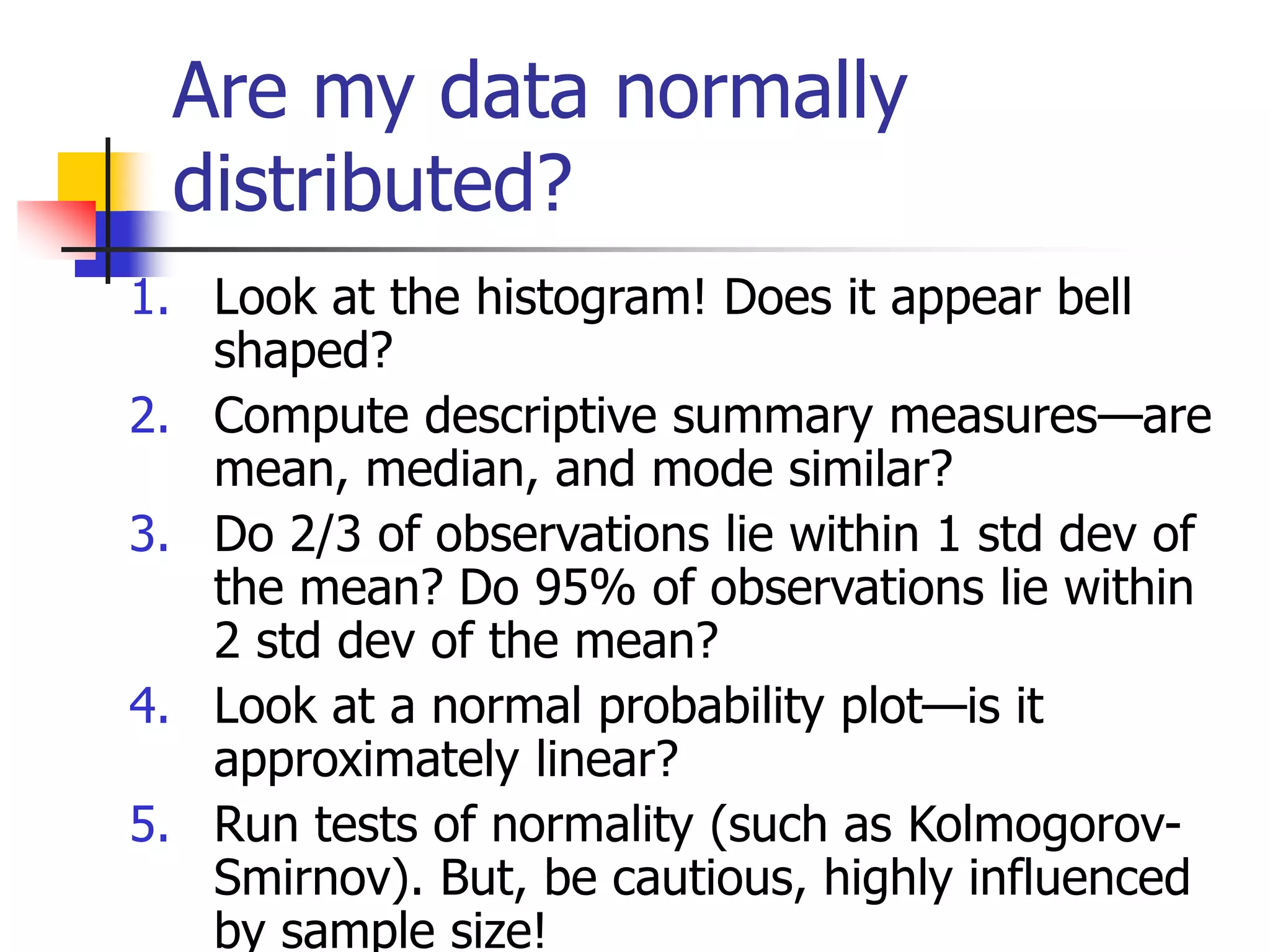
Are my datanormally
distributed?
1. Look at the histogram! Does it appear bell
shaped?
2. Compute descriptive summary measures—are
mean, median, and mode similar?
3. Do 2/3 of observations lie within 1 std dev of
the mean? Do 95% of observations lie within
2 std dev of the mean?
4. Look at a normal probability plot—is it
approximately linear?
5. Run tests of normality (such as Kolmogorov-
Smirnov). But, be cautious, highly influenced
by sample size!
27.
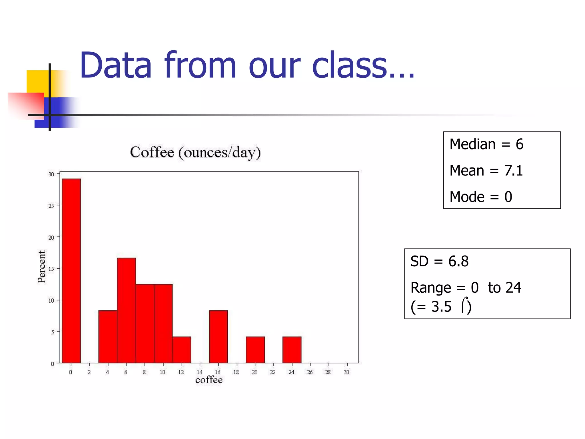
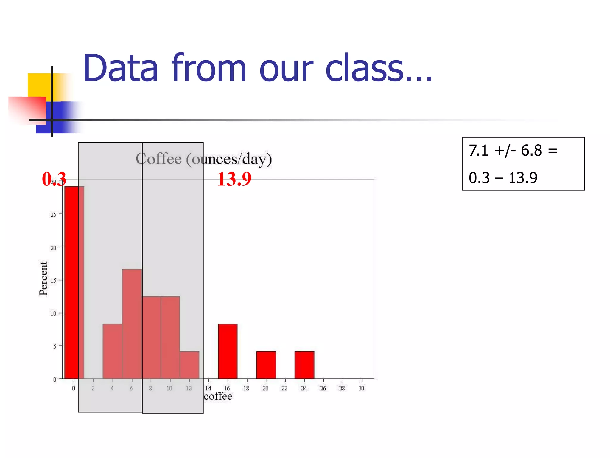
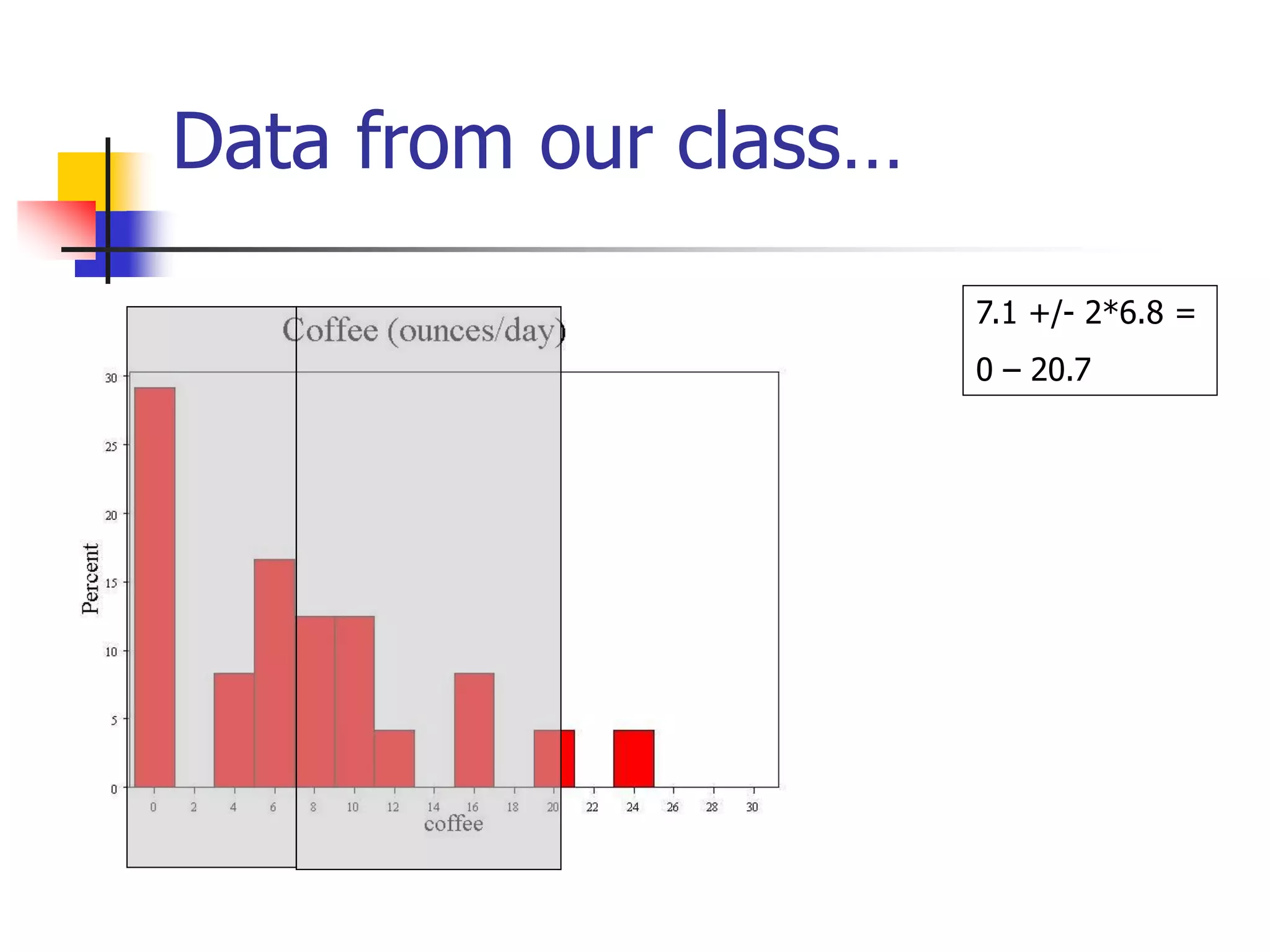
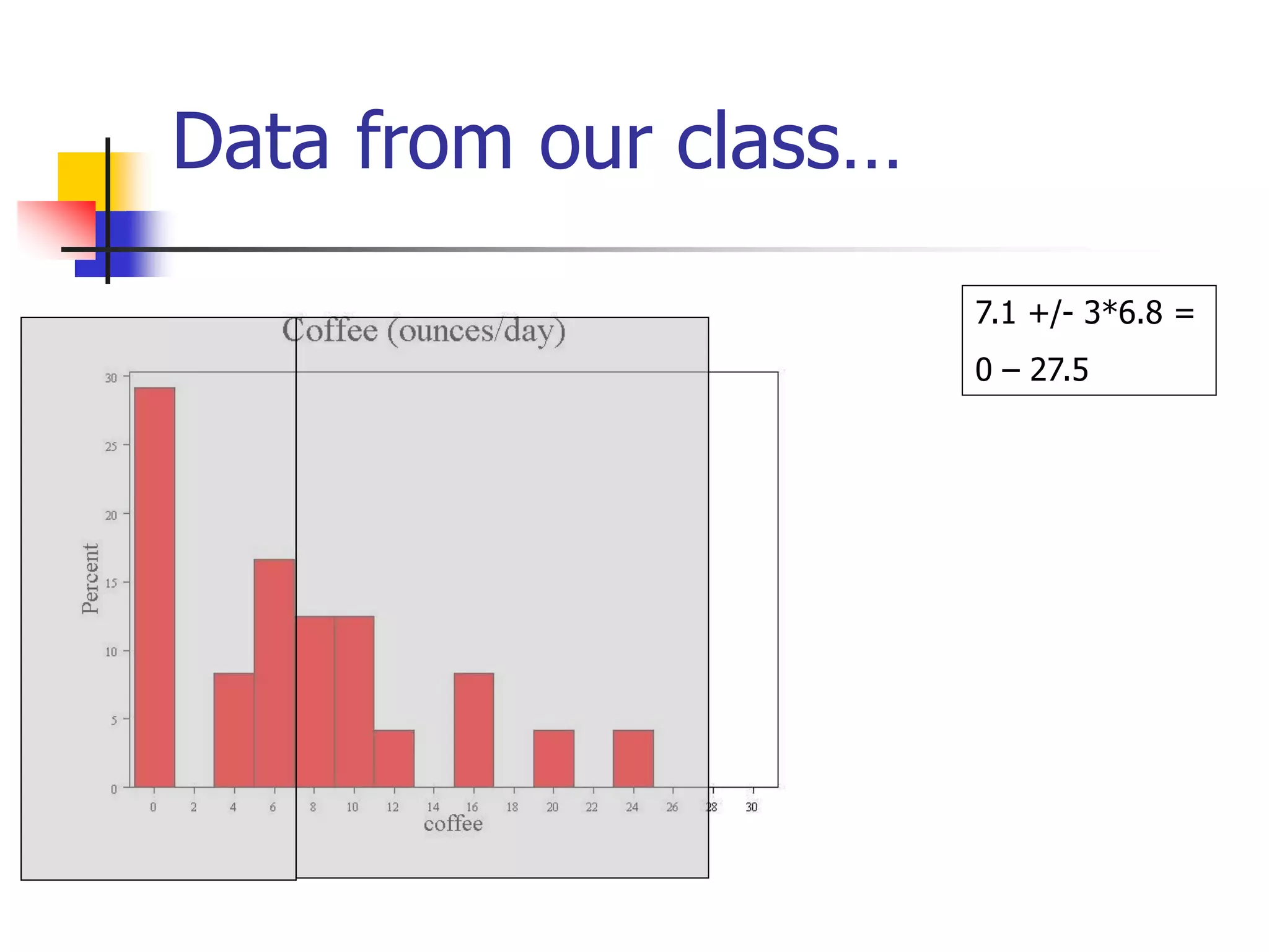
Data from ourclass…
Median = 6
Mean = 7.1
Mode = 0
SD = 6.8
Range = 0 to 24
(= 3.5 )
28.
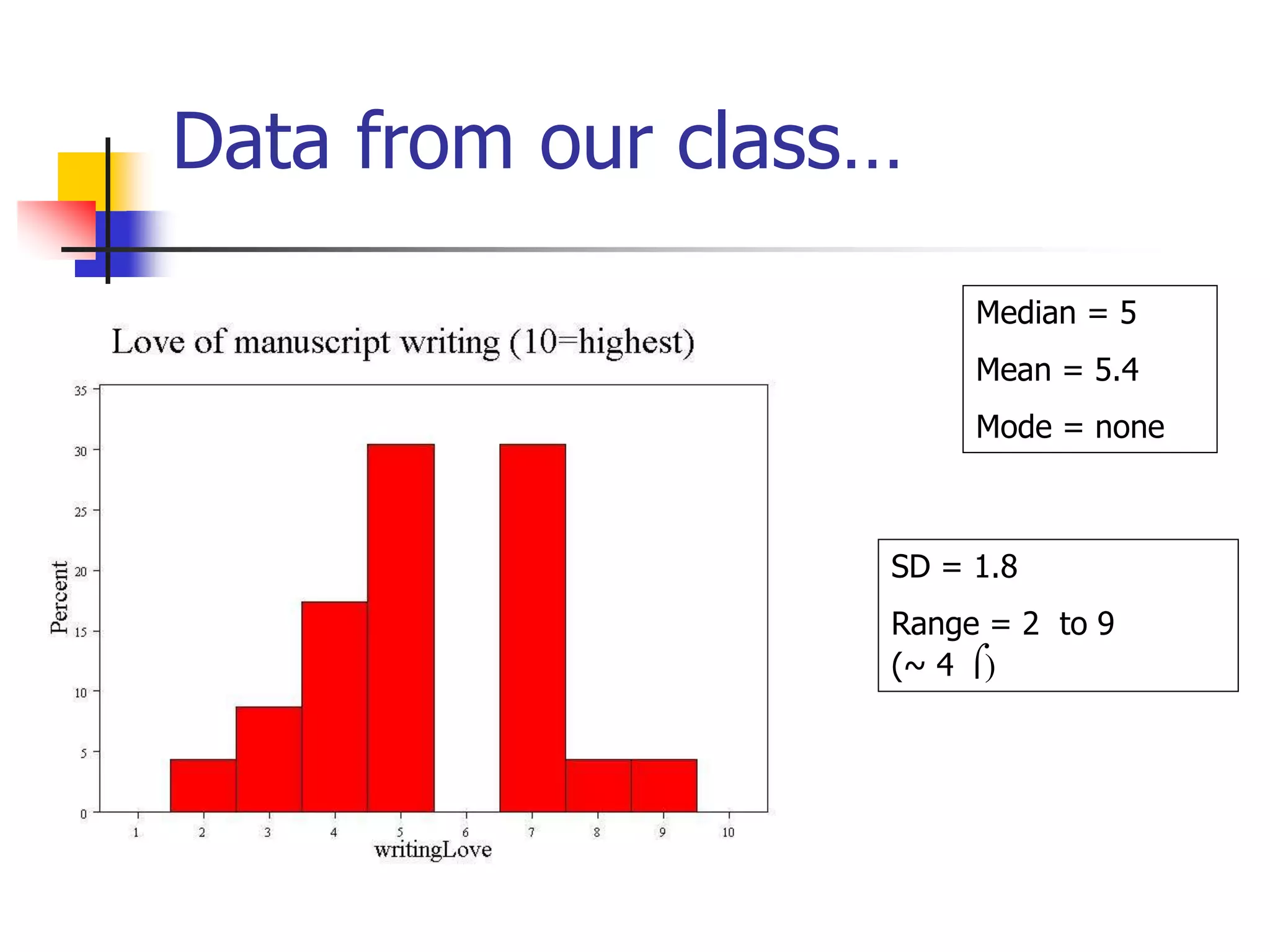
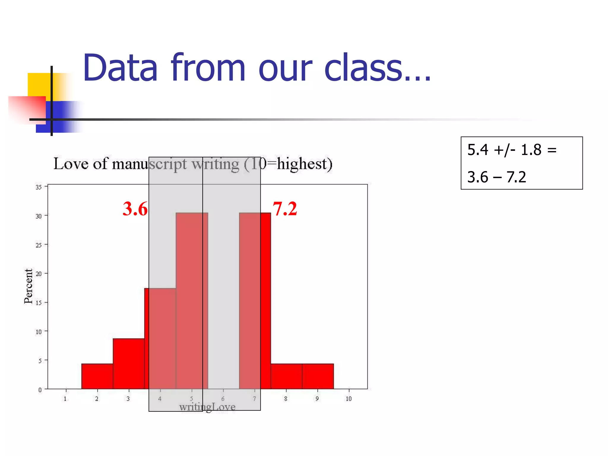
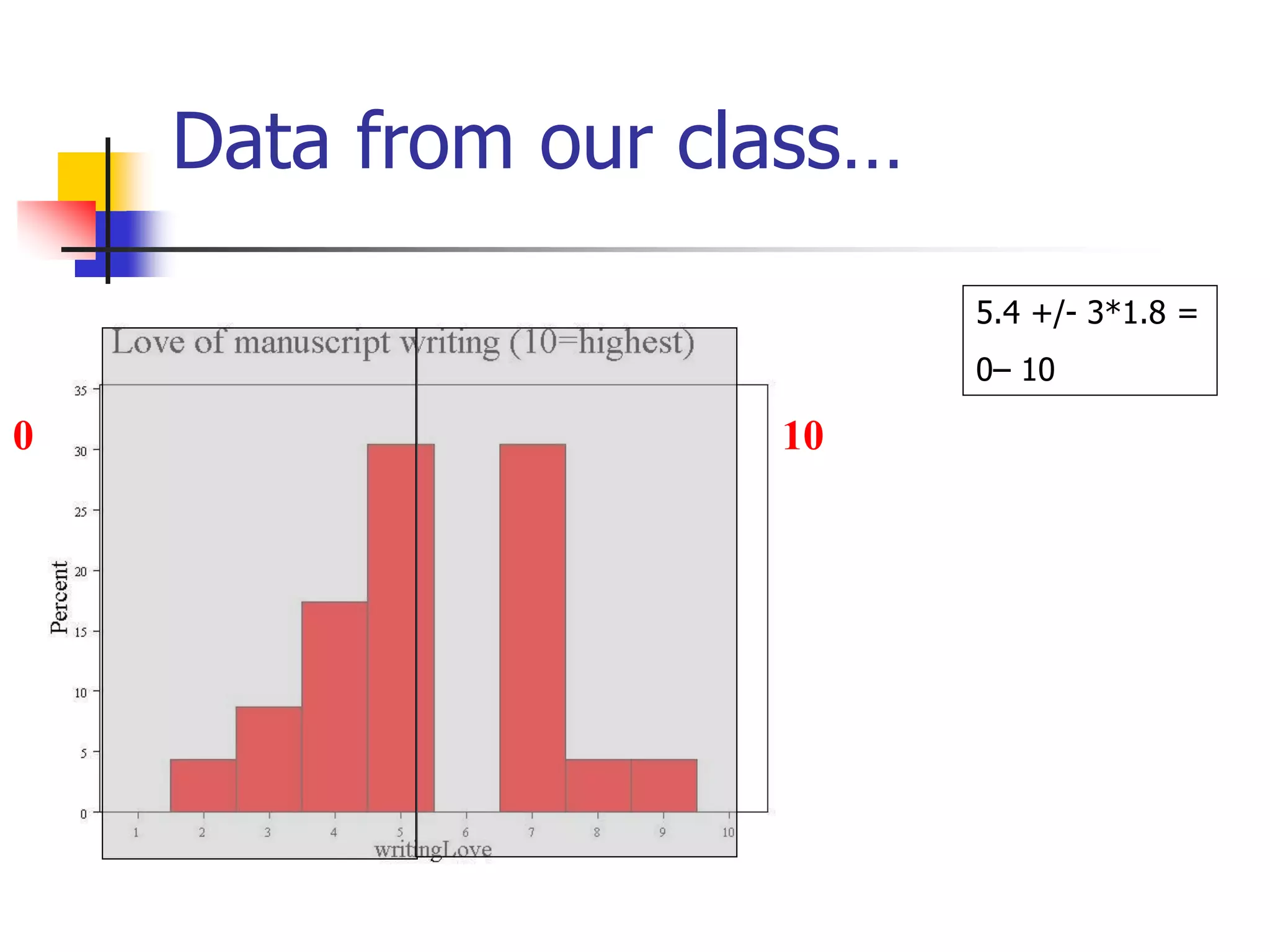
Data from ourclass…
Median = 5
Mean = 5.4
Mode = none
SD = 1.8
Range = 2 to 9
(~ 4 )
29.
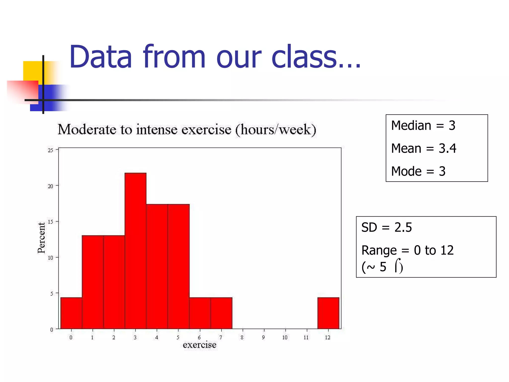
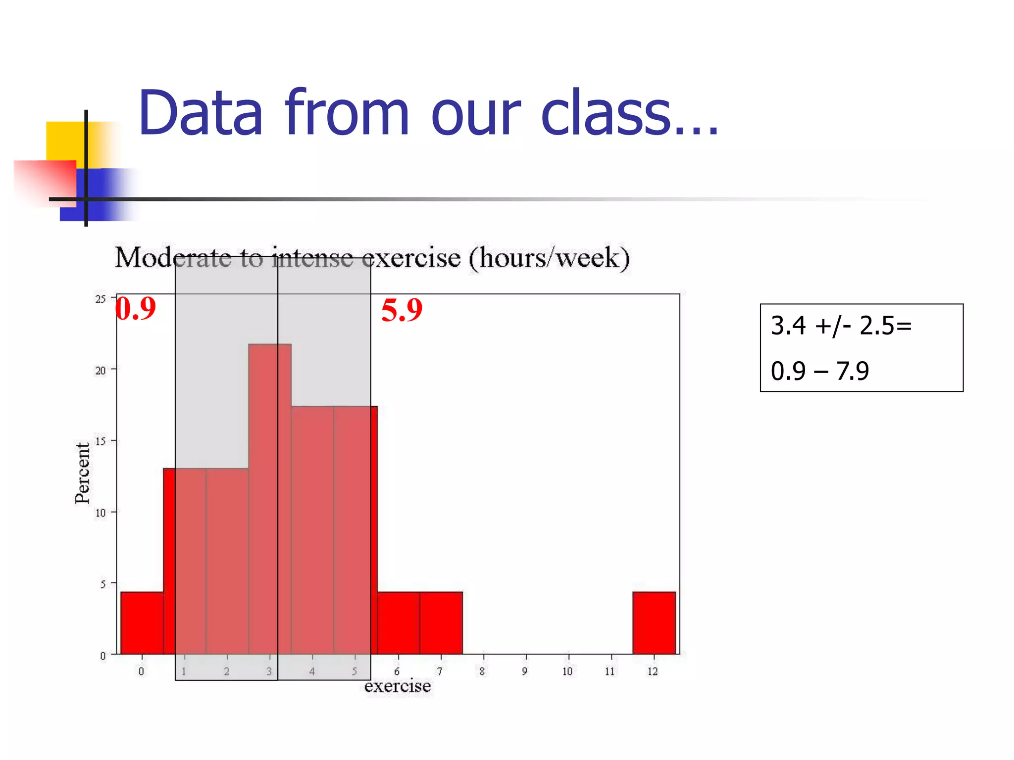
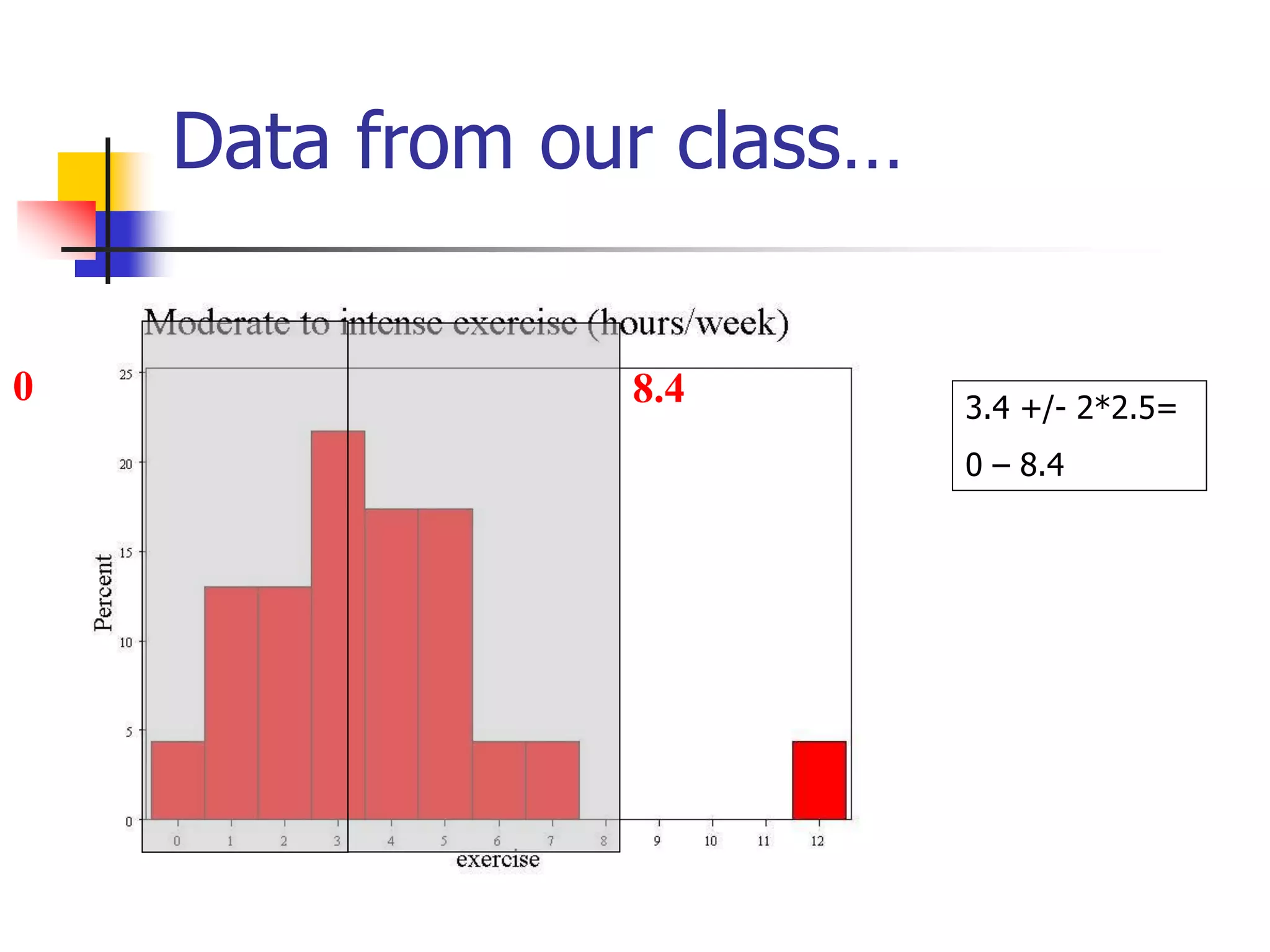
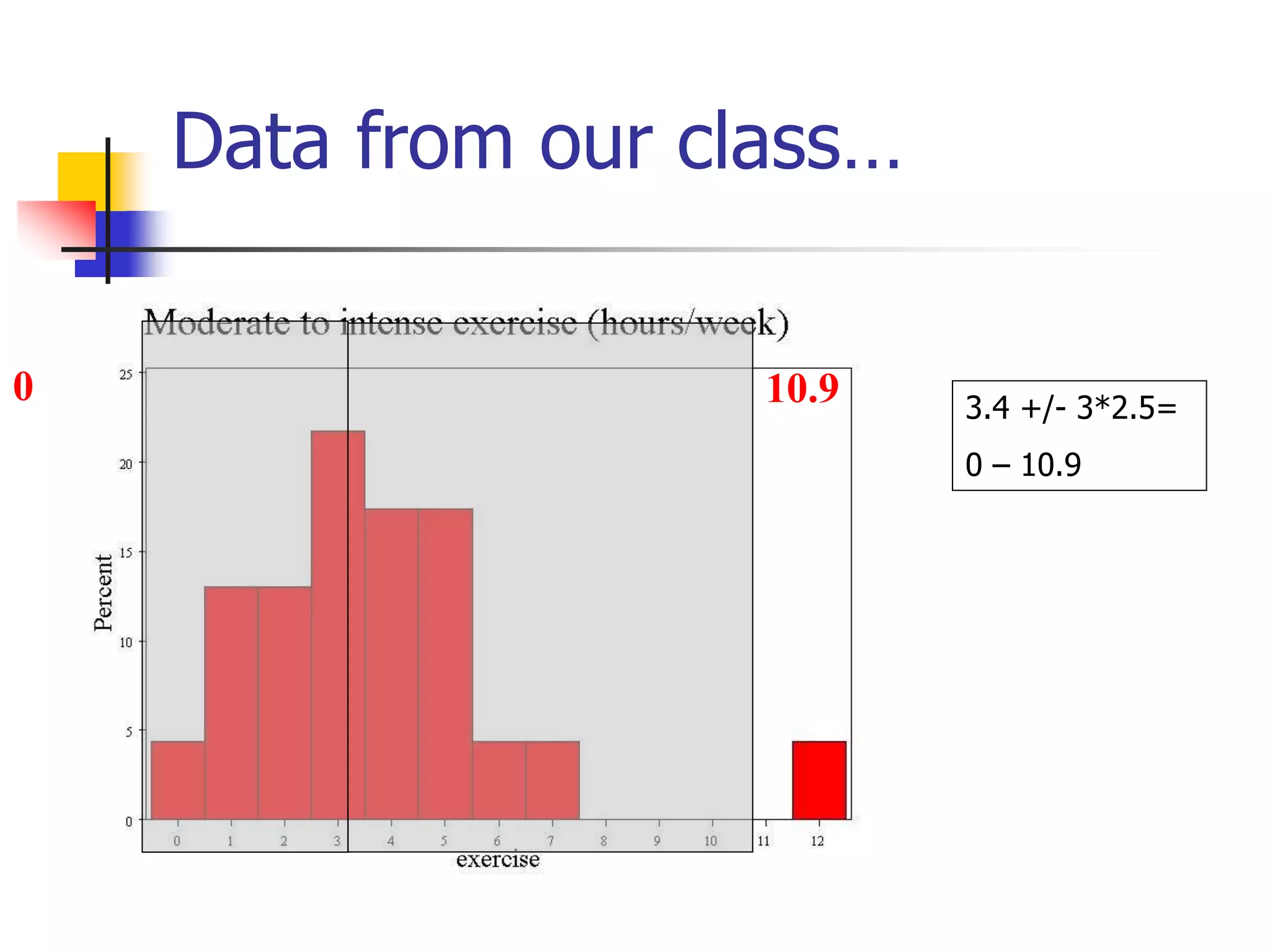
Data from ourclass…
Median = 3
Mean = 3.4
Mode = 3
SD = 2.5
Range = 0 to 12
(~ 5 )
30.
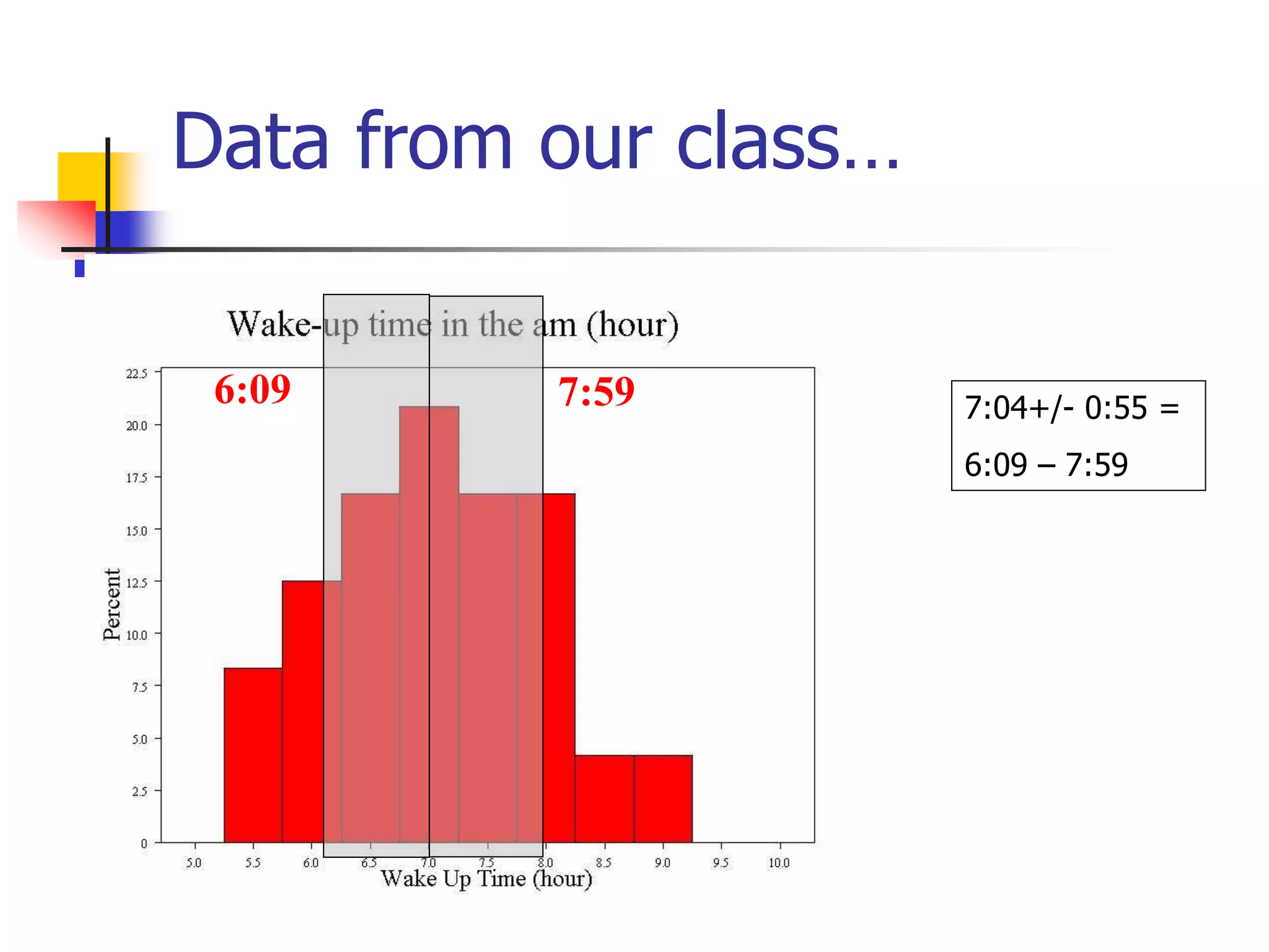
Data from ourclass…
Median = 7:00
Mean = 7:04
Mode = 7:00
SD = :55
Range = 5:30 to 9:00
(~4 )
31.
Data from ourclass…
7.1 +/- 6.8 =
0.3 – 13.9
0.3 13.9
Data from ourclass…
7:04+/- 0:55 =
6:09 – 7:59
6:09 7:59
41.
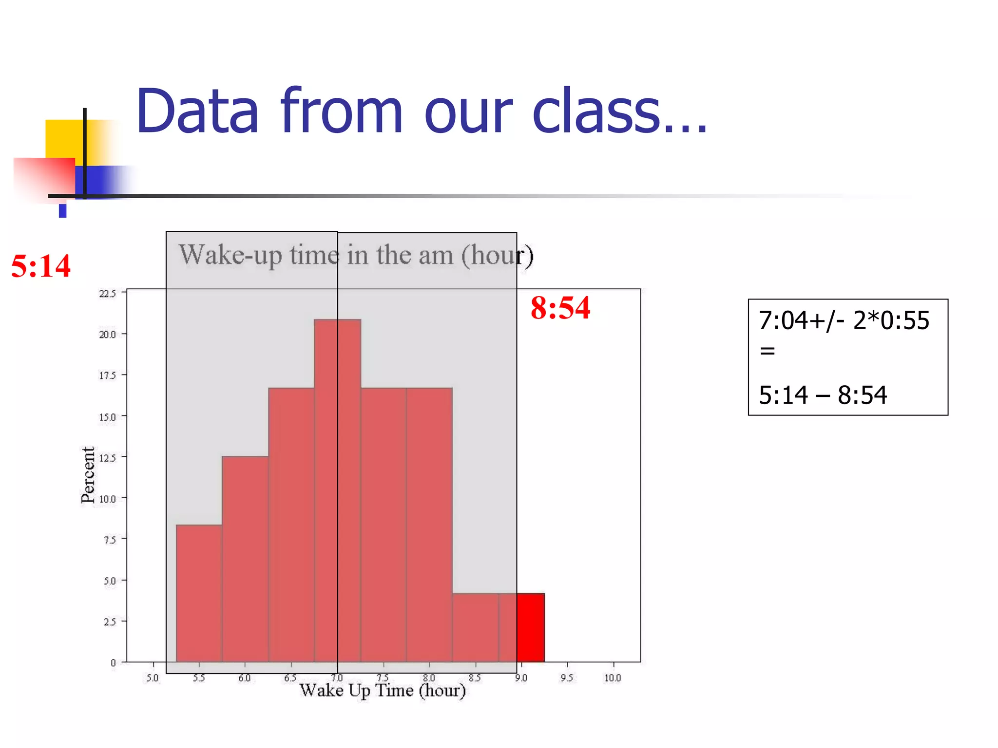
Data from ourclass…
7:04+/- 2*0:55
=
5:14 – 8:54
5:14
8:54
42.
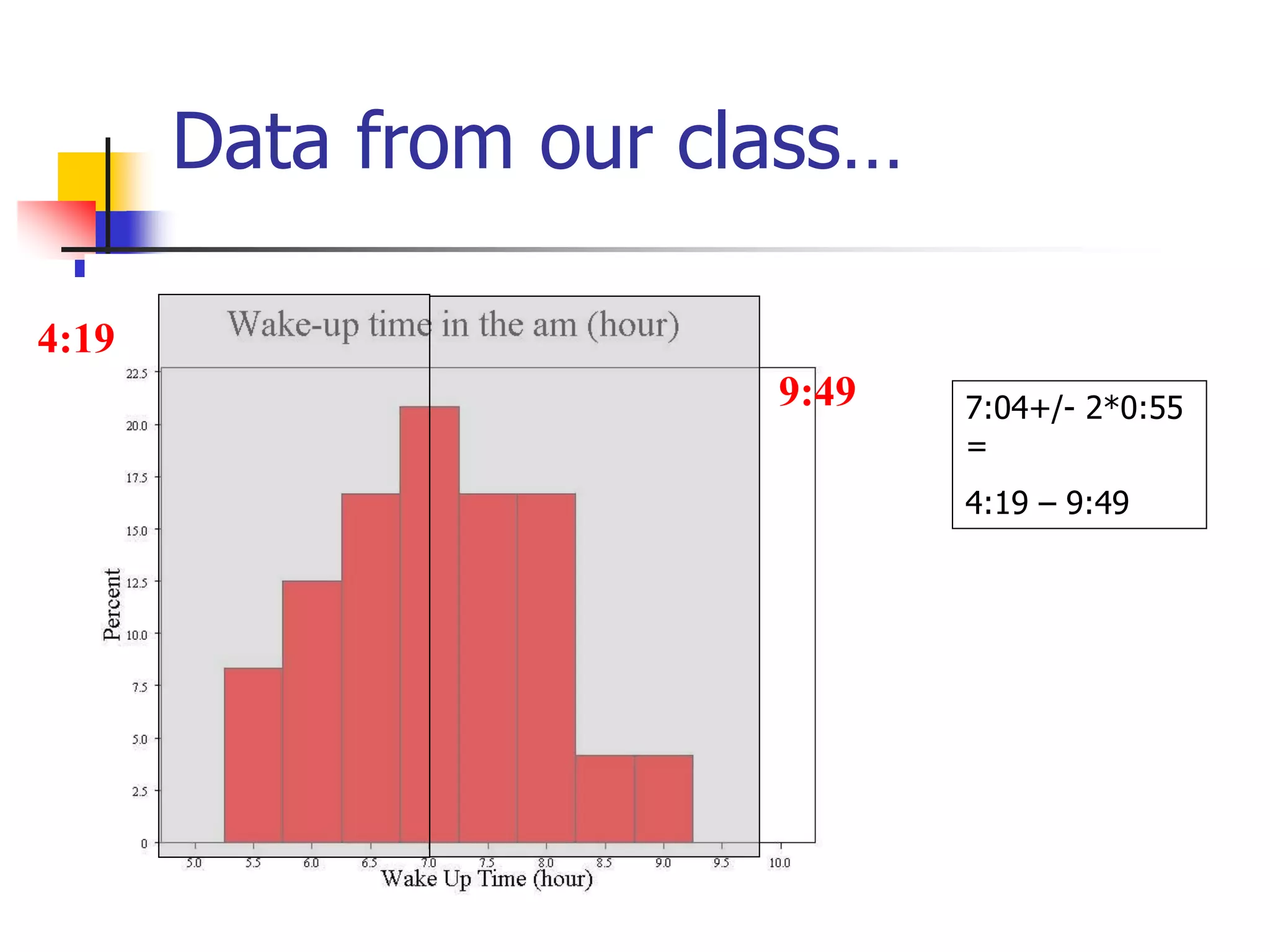
Data from ourclass…
7:04+/- 2*0:55
=
4:19 – 9:49
4:19
9:49
43.
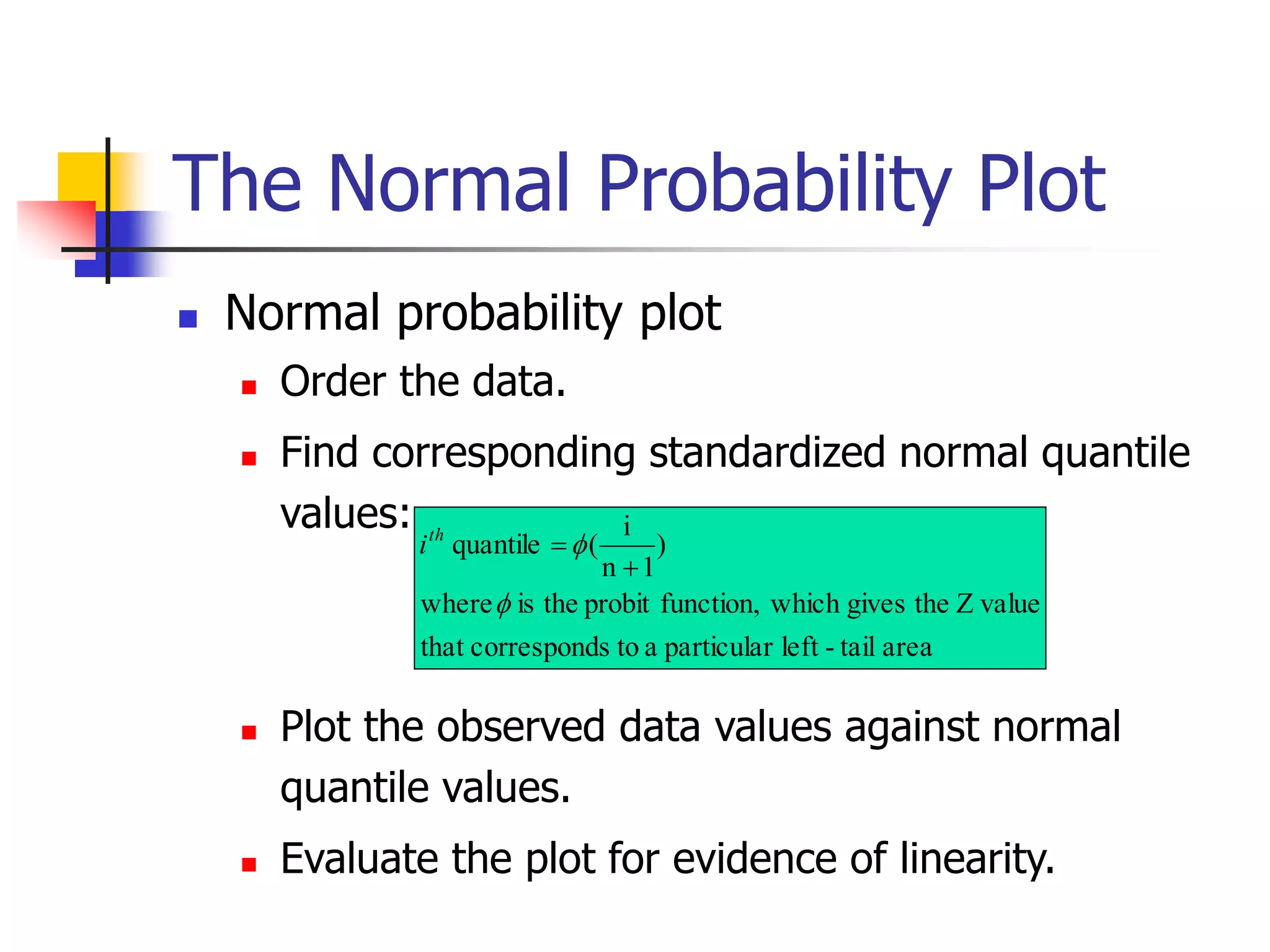
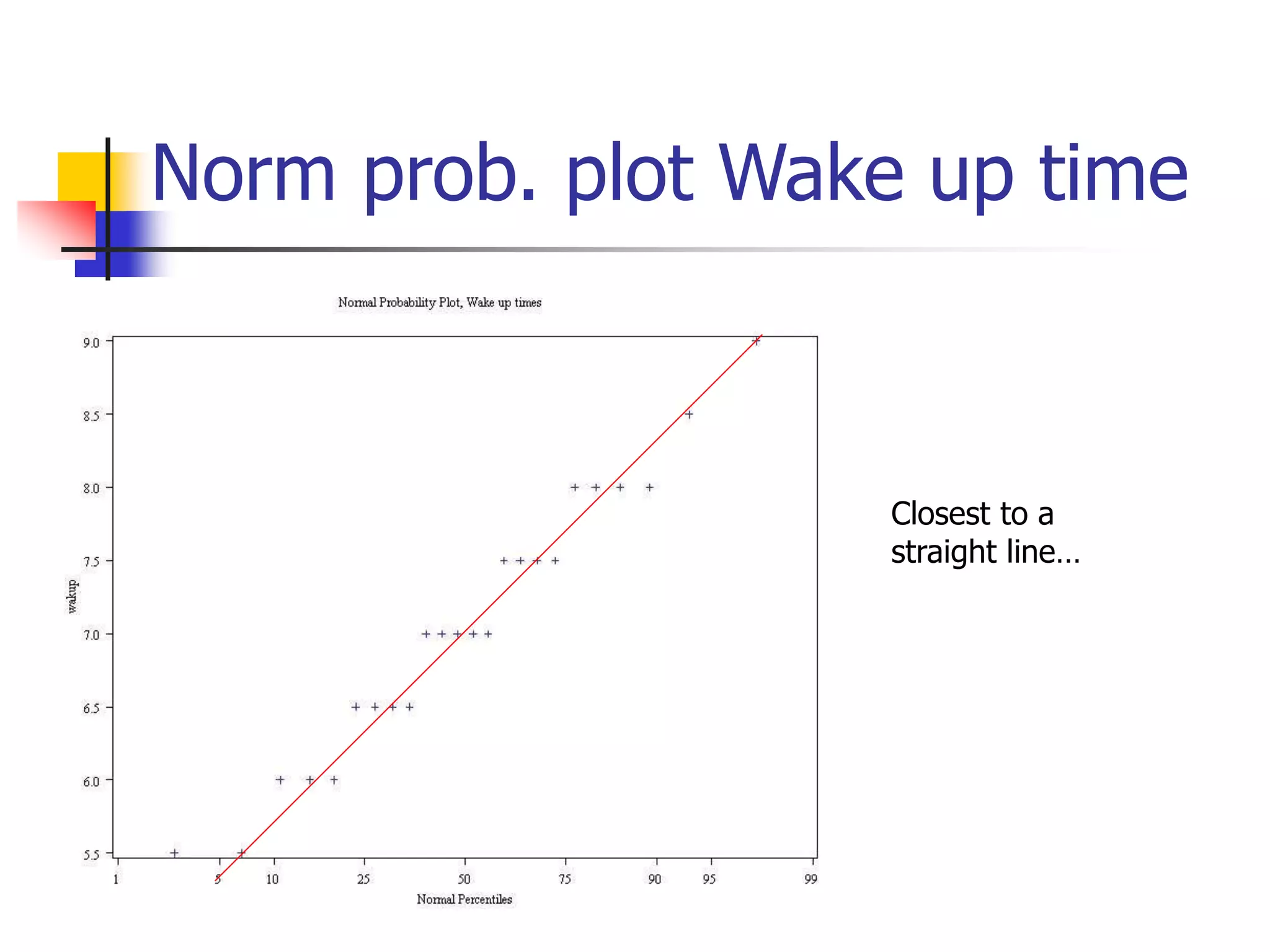
The Normal ProbabilityPlot
Normal probability plot
Order the data.
Find corresponding standardized normal quantile
values:
Plot the observed data values against normal
quantile values.
Evaluate the plot for evidence of linearity.
area
tail
-
left
particular
a
to
s
correspond
that
value
Z
the
gives
which
function,
probit
the
is
where
)
1
n
i
(
quantile
th
i
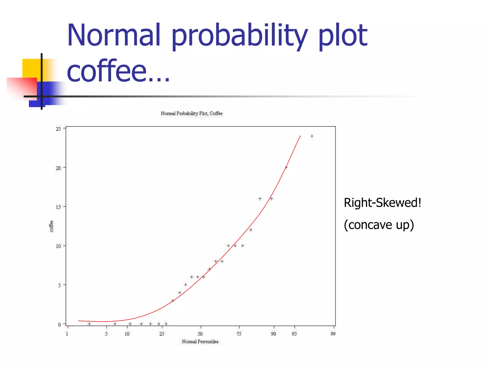
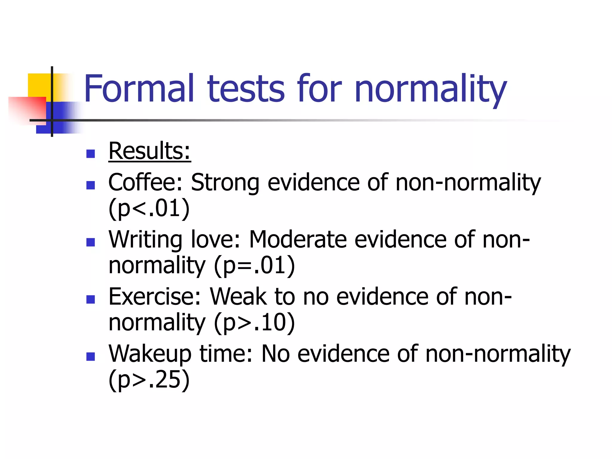
Formal tests fornormality
Results:
Coffee: Strong evidence of non-normality
(p<.01)
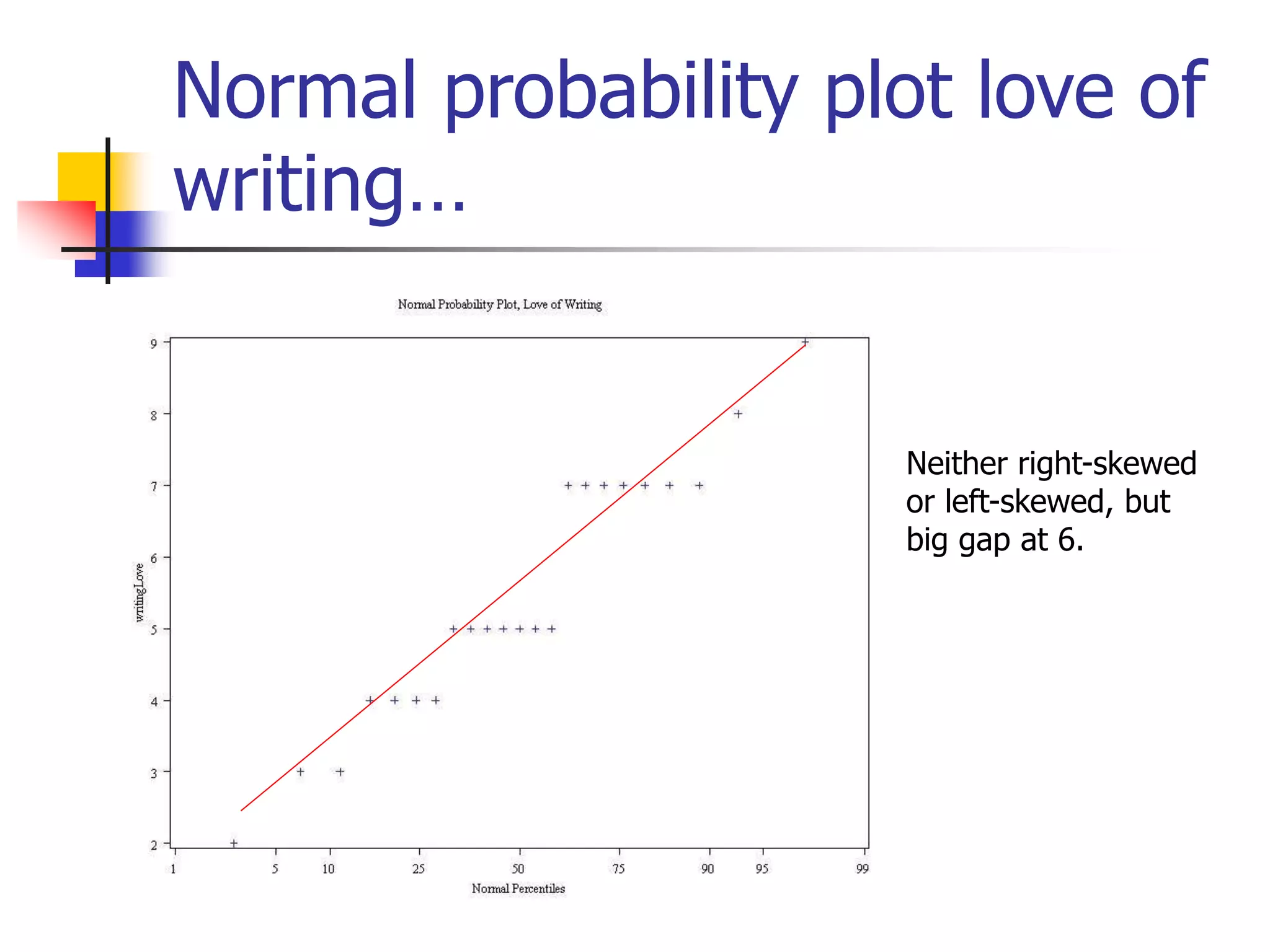
Writing love: Moderate evidence of non-
normality (p=.01)
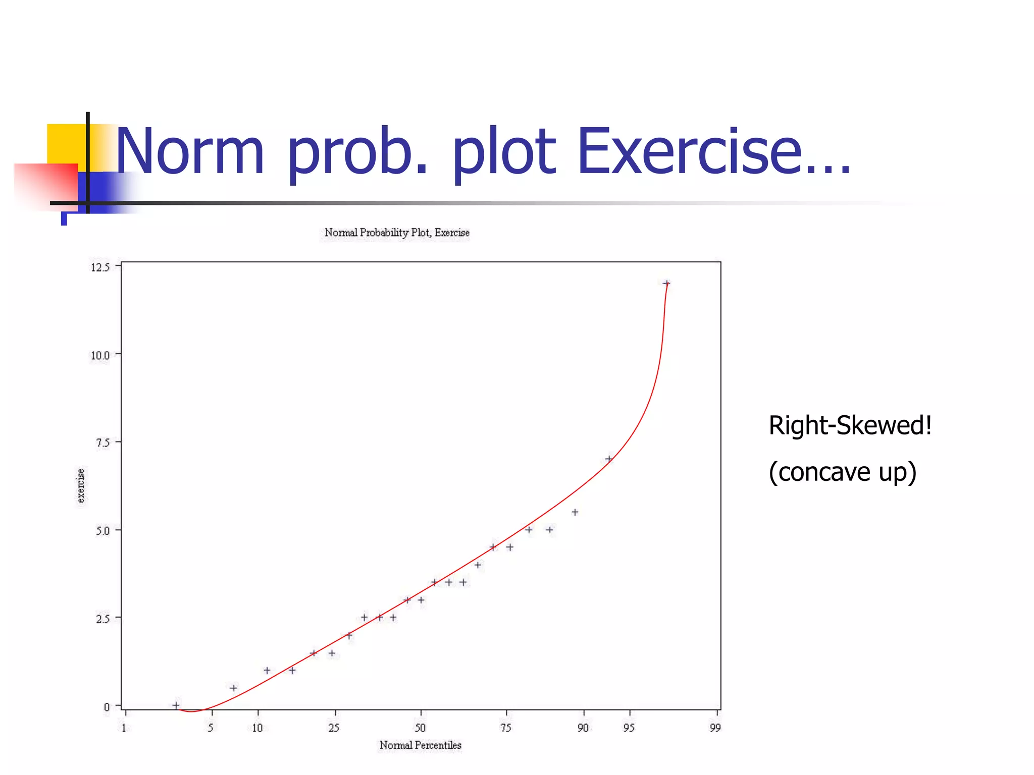
Exercise: Weak to no evidence of non-
normality (p>.10)
Wakeup time: No evidence of non-normality
(p>.25)
49.
Normal approximation tothe
binomial
When you have a binomial distribution where n is
large and p is middle-of-the road (not too small, not
too big, closer to .5), then the binomial starts to look
like a normal distribution in fact, this doesn’t even
take a particularly large n
Recall: What is the probability of being a smoker among
a group of cases with lung cancer is .6, what’s the
probability that in a group of 8 cases you have less
than 2 smokers?
50.
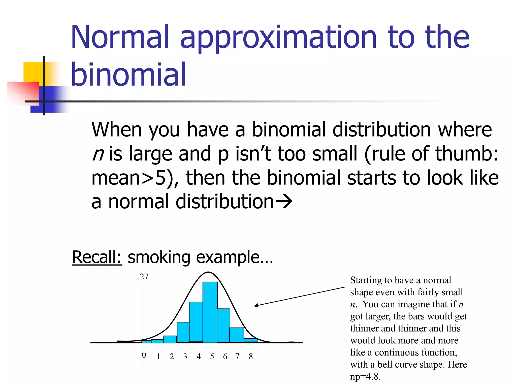
Normal approximation tothe
binomial
When you have a binomial distribution where
n is large and p isn’t too small (rule of thumb:
mean>5), then the binomial starts to look like
a normal distribution
Recall: smoking example…
1 4 5
2 3 6 7 8
0
.27 Starting to have a normal
shape even with fairly small
n. You can imagine that if n
got larger, the bars would get
thinner and thinner and this
would look more and more
like a continuous function,
with a bell curve shape. Here
np=4.8.
51.
Normal approximation to
binomial
14 5
2 3 6 7 8
0
.27
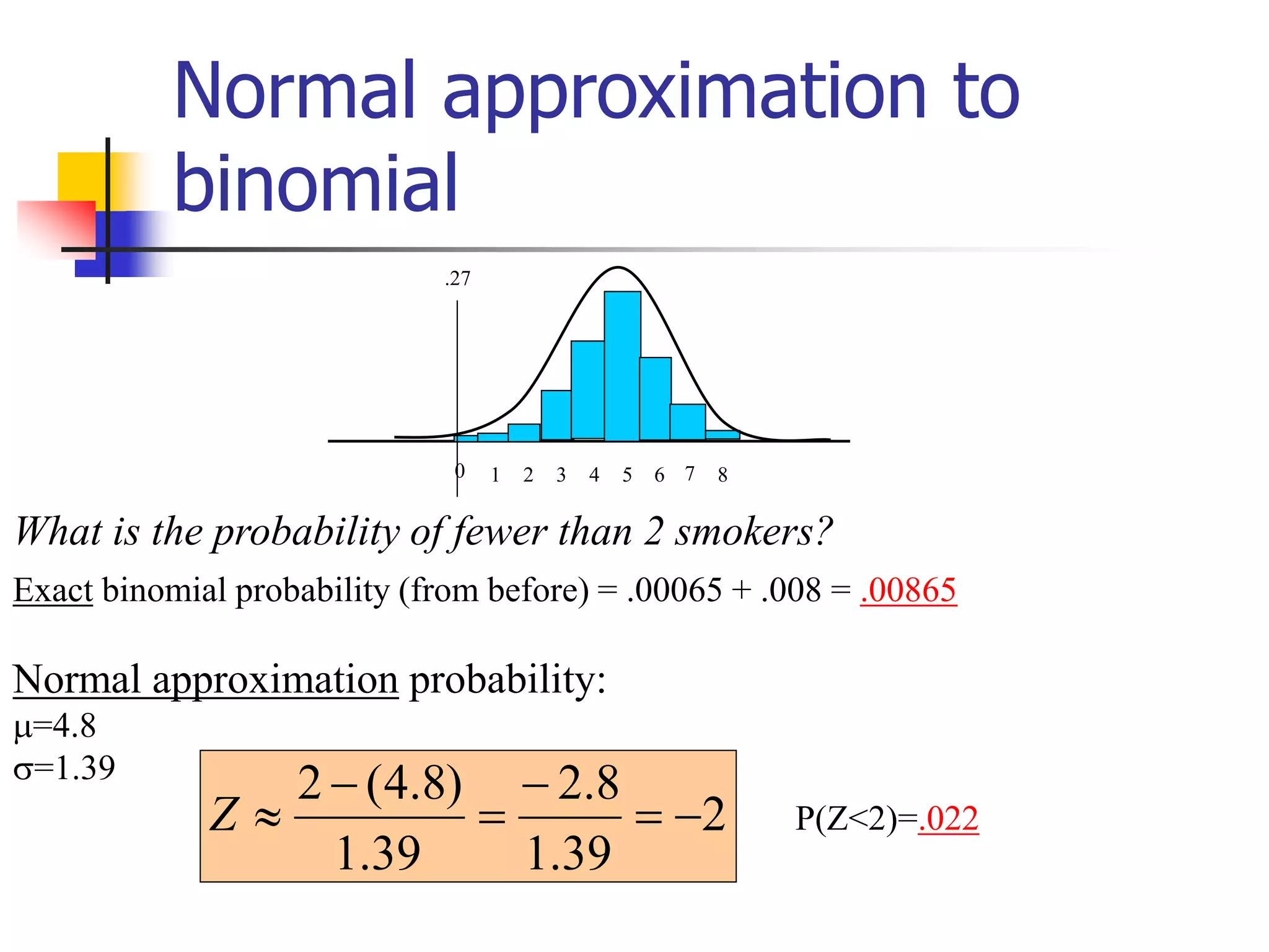
What is the probability of fewer than 2 smokers?
Normal approximation probability:
=4.8
=1.39
2
39
.
1
8
.
2
39
.
1
)
8
.
4
(
2
Z
Exact binomial probability (from before) = .00065 + .008 = .00865
P(Z<2)=.022
52.
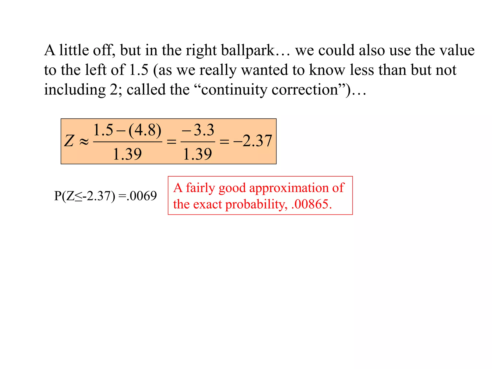
A little off,but in the right ballpark… we could also use the value
to the left of 1.5 (as we really wanted to know less than but not
including 2; called the “continuity correction”)…
37
.
2
39
.
1
3
.
3
39
.
1
)
8
.
4
(
5
.
1
Z
P(Z≤-2.37) =.0069
A fairly good approximation of
the exact probability, .00865.
53.
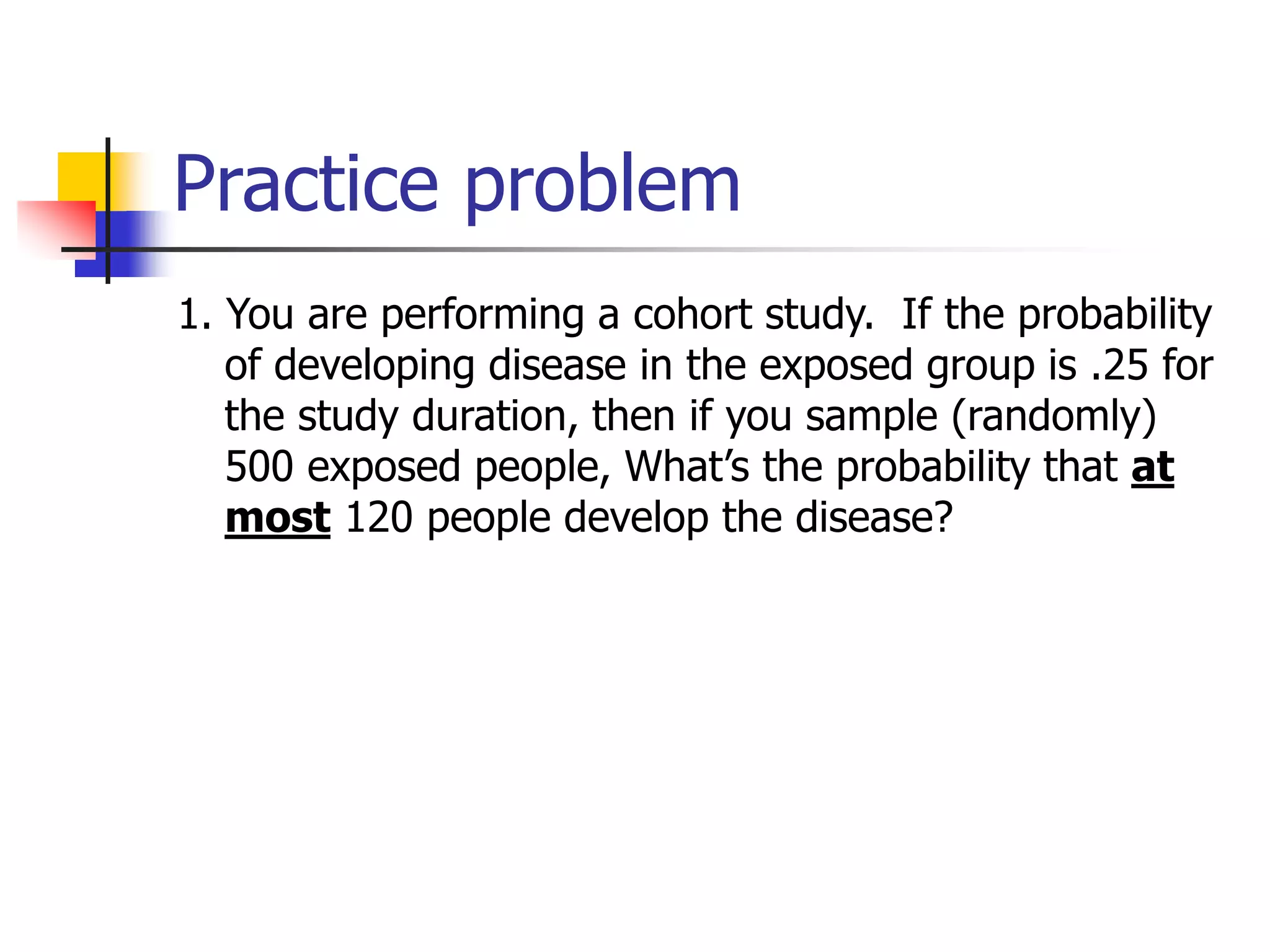
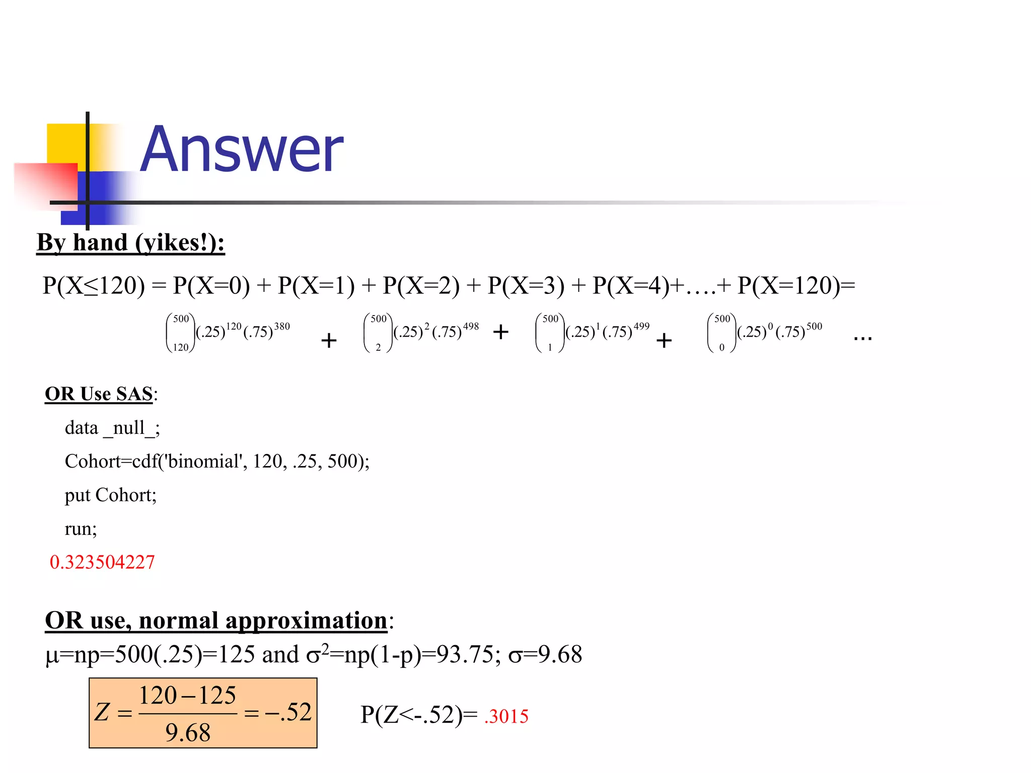
Practice problem
1. Youare performing a cohort study. If the probability
of developing disease in the exposed group is .25 for
the study duration, then if you sample (randomly)
500 exposed people, What’s the probability that at
most 120 people develop the disease?
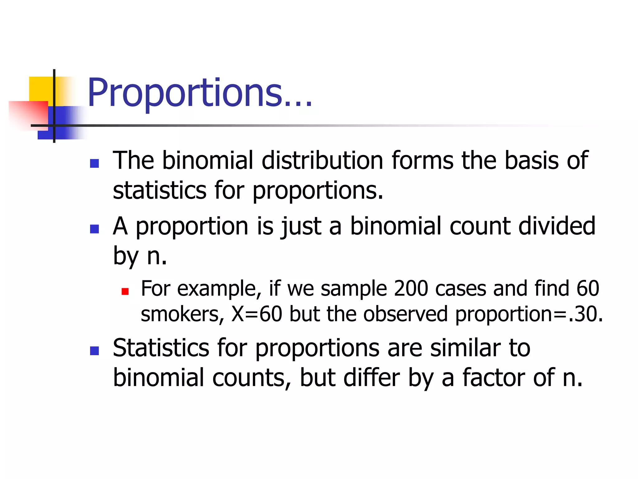
Proportions…
The binomialdistribution forms the basis of
statistics for proportions.
A proportion is just a binomial count divided
by n.
For example, if we sample 200 cases and find 60
smokers, X=60 but the observed proportion=.30.
Statistics for proportions are similar to
binomial counts, but differ by a factor of n.
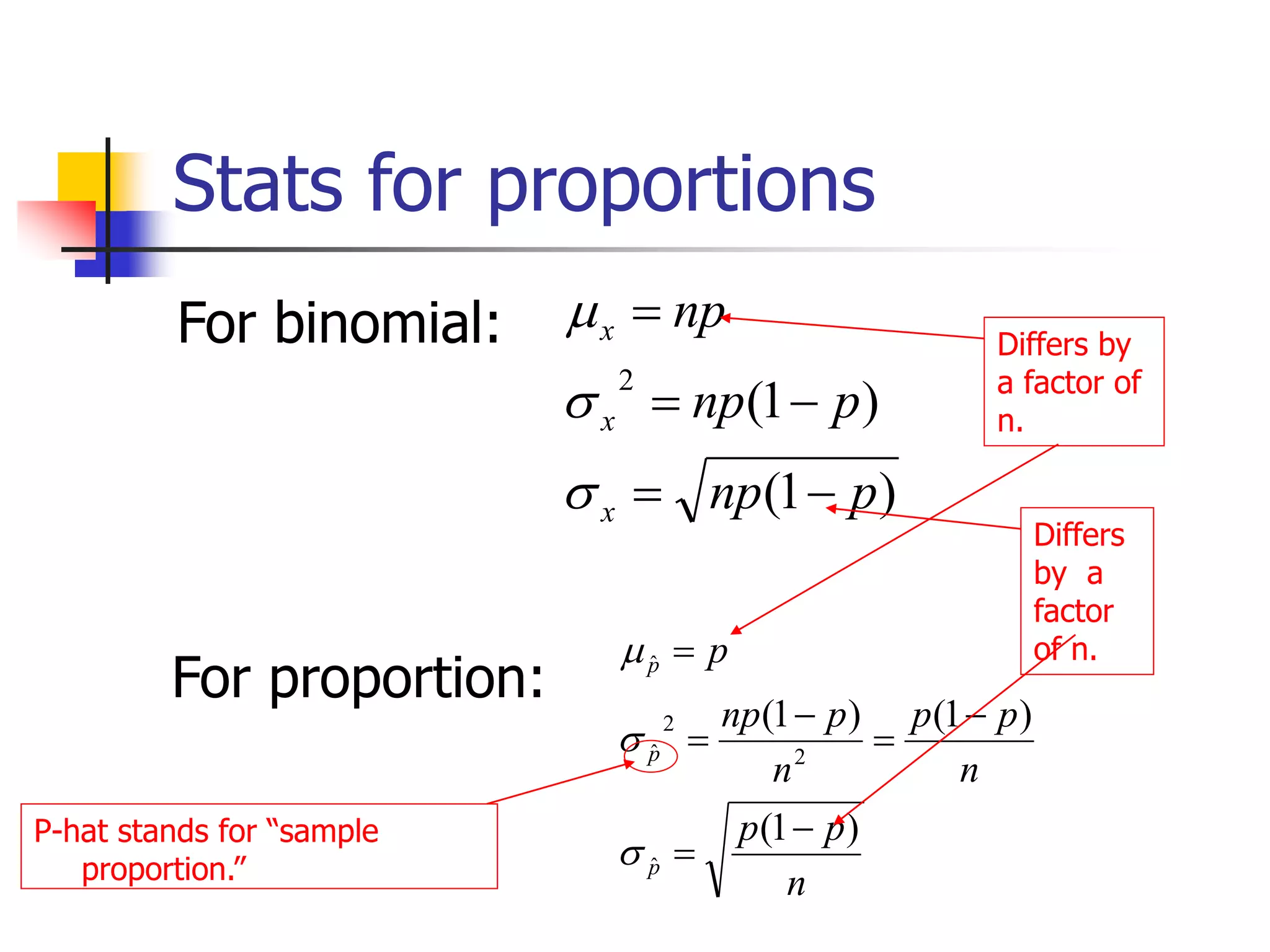
56.
Stats for proportions
Forbinomial:
)
1
(
)
1
(
2
p
np
p
np
np
x
x
x
For proportion:
n
p
p
n
p
p
n
p
np
p
p
p
p
)
1
(
)
1
(
)
1
(
ˆ
2
2
ˆ
ˆ
P-hat stands for “sample
proportion.”
Differs by
a factor of
n.
Differs
by a
factor
of n.
57.
It all comesback to Z…
Statistics for proportions are based on a
normal distribution, because the
binomial can be approximated as
normal if np>5