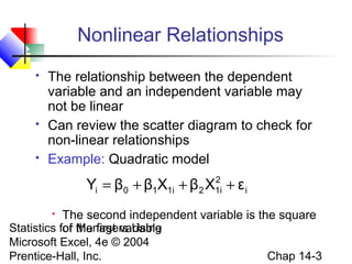
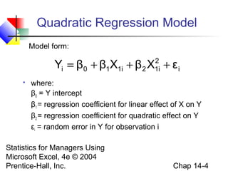
multiple regression model building

Statistics for Managers Using Microsoft Excel, 4e © 2004 Prentice-Hall, Inc. Chap 14-1
Chapter 14
Multiple Regression Model Building
Statistics for Managers
Using Microsoft®
Excel
4th
Edition

Statistics for Managers Using
Microsoft Excel, 4e © 2004
Prentice-Hall, Inc. Chap 14-2
Chapter Goals
After completing this chapter, you should be
able to:
 use quadratic terms in a regression model
 use transformed variables in a regression model
 measure the correlation among the independent
variables
 build a regression model using either the stepwise or
best-subsets approach
 explain the pitfalls involved in developing a multiple
regression model

 The relationship between the dependent
variable and an independent variable may
not be linear
 Can review the scatter diagram to check for
non-linear relationships
 Example: Quadratic model
 The second independent variable is the square
of the first variable
Nonlinear Relationships
i
2
1i21i10i εXβXββY +++=

Quadratic Regression Model
 where:
β0 = Y intercept
β1 = regression coefficient for linear effect of X on Y
β2 = regression coefficient for quadratic effect on Y
εi = random error in Y for observation i
i
2
Model form:

Linear fit does not give
random residuals
Linear vs. Nonlinear Fit
Nonlinear fit gives
random residuals

X
residuals
X
Y
X
residuals
Y
X

Quadratic Regression Model
Quadratic models may be considered when the scatter
diagram takes on one of the following shapes:
X1
Y
X1X1
YYY
β1 < 0 β1 > 0 β1 < 0 β1 > 0
β1 = the coefficient of the linear term
β2 = the coefficient of the squared term
X1
i
2
β2 > 0 β2 > 0 β2 < 0 β2 < 0

Testing the Overall
Quadratic Model
 Test for Overall Relationship
H0: β1 = β2 = 0 (no overall relationship between X and Y)
H1: β1 and/or β2 ≠ 0 (there is a relationship between X and Y)
 F test statistic =
2
1i21i10i XbXbbYˆ ++=
MSE
MSR
 Estimate the quadratic model to obtain the
regression equation:

Testing for Significance:
Quadratic Effect
 Testing the Quadratic Effect
 Compare quadratic regression equation
with the linear regression equation
2
1i21i10i XbXbbY ++=
1i10i XbbY +=

Quadratic Effect
 Consider the quadratic regression equaiton
Hypotheses

(The quadratic term does not improve the model)

(The quadratic term improves the model)
2
1i21i10i XbXbbY ++=
H0: β2 = 0
H1: β2 ≠ 0
(continued)

Quadratic Effect
Hypotheses

(The quadratic term does not improve the model)

(The quadratic term improves the model)
 The test statistic is
H0: β2 = 0
H1: β2 ≠ 0
(continued)
2b
22
S
βb
t
−
=
3nd.f. −=
where:
b2 = squared term slope
coefficient
β2 = hypothesized slope (zero)
Sb = standard error of the slope2

Quadratic Effect
Compare r2
from simple regression to
adjusted r2
from the quadratic model
 If adj. r2
from the quadratic model is larger
than the r2
from the simple model, then the
quadratic model is a better model
(continued)

Example: Quadratic Model
 Purity increases as filter time
increases:
Purity
Filter
Time
3 1
7 2
8 3
15 5
22 7
33 8
40 10
54 12
67 13
70 14
78 15
85 15
87 16
99 17
Purity vs. Time
0
20
40
60
80
100
0 5 10 15 20
Time
Purity

(continued)
Regression Statistics
R Square 0.96888
Adjusted R Square 0.96628
Standard Error 6.15997
 Simple regression results:
Y = -11.283 + 5.985 Time
Coefficients
Standard
Error t Stat P-value
Intercept -11.28267 3.46805 -3.25332 0.00691
Time 5.98520 0.30966 19.32819 2.078E-10
F Significance F
373.57904 2.0778E-10
^
Time Residual Plot
-10
-5
0
5
10
0 5 10 15 20
Time
Residuals
t statistic, F statistic, and r2
are all high, but the
residuals are not random:

Coefficients
Standard
Error t Stat P-value
Intercept 1.53870 2.24465 0.68550 0.50722
Time 1.56496 0.60179 2.60052 0.02467
Time-squared 0.24516 0.03258 7.52406 1.165E-05
R Square 0.99494
Adjusted R Square 0.99402
F Significance F
1080.7330 2.368E-13
 Quadratic regression results:
Y = 1.539 + 1.565 Time + 0.245 (Time)2
^
(continued)
Time Residual Plot
-5
0
5
10
0 5 10 15 20
Time
Residuals
Time-squared Residual Plot
-5
0
5
10
0 100 200 300 400
Time-squared
Residuals
The quadratic term is significant and
improves the model: adj. r2
is higher and
SYX is lower, residuals are now random

Using Transformations in
Regression Analysis
Idea:
 non-linear models can often be transformed
to a linear form
 Can be estimated by least squares if transformed
 transform X or Y or both to get a better fit or
to deal with violations of regression
assumptions
 Can be based on theory, logic or scatter
diagrams

The Square Root Transformation
 The square-root transformation
 Used to
 overcome violations of the homoscedasticity
assumption
 fit a non-linear relationship
i1i10i εXββY ++=

 Shape of original relationship
X
The Square Root Transformation
(continued)
b1 > 0
b1 < 0
X
Y
Y
Y
Y
X
X
 Relationship when transformed
i1i10i εXββY ++=i1i10i εXββY ++=

 Original multiplicative model
The Log Transformation
 Transformed multiplicative model
i
β
1i0i εXβY 1
= i1i10i εlogXlogββlogYlog ++=
The Multiplicative Model:
 Original multiplicative model  Transformed exponential model
i2i21i10i εlnXβXββYln +++=
The Exponential Model:
i
XβXββ
i εeY 2i21i10 ++
=

Interpretation of coefficients
For the multiplicative model:
 When both dependent and independent
variables are logged:
 The coefficient of the independent variable Xk can
be interpreted as : a 1 percent change in Xk leads to
an estimated bk percentage change in the average
value of Y. Therefore bk is the elasticity of Y with
respect to a change in Xk .
i1i10i εlogXlogββlogYlog ++=

Collinearity
 Collinearity: High correlation exists among two
or more independent variables
 This means the correlated variables contribute
redundant information to the multiple regression
model

Collinearity
 Including two highly correlated explanatory
variables can adversely affect the regression
results
 No new information provided
 Can lead to unstable coefficients (large
standard error and low t-values)
 Coefficient signs may not match prior
expectations
(continued)

Some Indications of
Strong Collinearity
 Incorrect signs on the coefficients
 Large change in the value of a previous
coefficient when a new variable is added to the
model
 A previously significant variable becomes
insignificant when a new independent variable
is added
 The estimate of the standard deviation of the
model increases when a variable is added to
the model

Detecting Collinearity
(Variance Inflationary Factor)
VIFj is used to measure collinearity:
If VIFj > 5, Xj is highly correlated with
the other explanatory variables
where R2
j is the coefficient of determination
of variable Xj with all other X variables
2
j
j
R1
1
VIF
−
=

Example: Pie Sales
Sales = b0 + b1 (Price)
+ b2 (Advertising)
Week
Pie
Sales
Price
($)
Advertising
($100s)
1 350 5.50 3.3
2 460 7.50 3.3
3 350 8.00 3.0
4 430 8.00 4.5
5 350 6.80 3.0
6 380 7.50 4.0
7 430 4.50 3.0
8 470 6.40 3.7
9 450 7.00 3.5
10 490 5.00 4.0
11 340 7.20 3.5
12 300 7.90 3.2
13 440 5.90 4.0
14 450 5.00 3.5
15 300 7.00 2.7
Recall the multiple regression
equation of chapter 13:

Detect Collinearity in PHStat
Output for the pie sales example:
 Since there are only two
explanatory variables, only one
VIF is reported

VIF is < 5

There is no evidence of
collinearity between Price and
Advertising
Regression Analysis
Price and all other X
Multiple R 0.030438
R Square 0.000926
Adjusted R
Square -0.075925
Observations 15
VIF 1.000927
PHStat / regression / multiple regression …
Check the “variance inflationary factor (VIF)” box

Model Building
 Goal is to develop a model with the best set of
independent variables
 Easier to interpret if unimportant variables are
removed
 Lower probability of collinearity
 Stepwise regression procedure
 Provide evaluation of alternative models as variables
are added
 Best-subset approach
 Try all combinations and select the best using the
highest adjusted r2
and lowest standard error

 Idea: develop the least squares regression
equation in steps, adding one explanatory
variable at a time and evaluating whether
existing variables should remain or be removed
 The coefficient of partial determination is the
measure of the marginal contribution of each
independent variable, given that other
independent variables are in the model
Stepwise Regression

Best Subsets Regression
 Idea: estimate all possible regression equations
using all possible combinations of independent
variables
 Choose the best fit by looking for the highest
adjusted r2
and lowest standard error
Stepwise regression and best subsets
regression can be performed using PHStat

Alternative Best Subsets
Criterion
 Calculate the value Cp for each potential
regression model
 Consider models with Cp values close to or
below k + 1
 k is the number of independent variables in the
model under consideration

Alternative Best Subsets
Criterion
 The Cp Statistic
))1k(2n(
R1
)Tn)(R1(
C 2
T
2
k
p +−−
−
−−
=
Where k = number of independent variables included in a
particular regression model
T = total number of parameters to be estimated in the
full regression model
= coefficient of multiple determination for model with k
independent variables
= coefficient of multiple determination for full model with
all T estimated parameters
2
kR
2
TR
(continued)

10 Steps in Model Building
1. Choose explanatory variables to include in the
model
2. Estimate full model and check VIFs
3. Check if any VIFs > 5
4.
 If no VIF > 5, go to step 5
 If one VIF > 5, remove this variable
 If more than one, eliminate the variable with the
highest VIF and go back to step 2
5. Perform best subsets regression with
remaining variables …

10 Steps in Model Building
6. List all models with Cp close to or less than (k
+ 1)
7. Choose the best model
 Consider parsimony
 Do extra variable make a significant contribution?
8. Perform complete analysis with chosen model,
including residual analysis
9. Transform the model if necessary to deal with
violations of linearity or other model
assumptions
10. Use the model for prediction
(continued)

Model Building Flowchart
Choose X1,X2,…Xk
Run regression
to find VIFs
Remove
variable with
highest
VIF
Any
VIF>5?
Run subsets
regression to obtain
“best” models in
terms of Cp
Do complete analysis
Add quadratic term and/or
transform variables as indicated
Perform
predictions
No
More
than one?
Remove
this X
Yes
No
Yes

Pitfalls and Ethical
Considerations
 Understand that interpretation of the
estimated regression coefficients are
performed holding all other independent
variables constant
 Evaluate residual plots for each independent
variable
 Evaluate interaction terms
To avoid pitfalls and address ethical considerations:

Additional Pitfalls
and Ethical Considerations
 Obtain VIFs for each independent variable
before determining which variables should be
included in the model
 Examine several alternative models using best-
subsets regression
 Use other methods when the assumptions
necessary for least-squares regression have
been seriously violated
To avoid pitfalls and address ethical considerations:
(continued)

Chapter Summary
 Developed the quadratic regression model
 Discussed using transformations in
regression models
 The multiplicative model
 The exponential model
 Described collinearity
 Discussed model building
 Stepwise regression
 Best subsets
 Addressed pitfalls in multiple regression and
ethical considerations

multiple regression model building

More Related Content

What's hot

Similar to multiple regression model building

More from Yesica Adicondro

Recently uploaded

multiple regression model building