DBM/380 v14
Create a Database
DBM/380 v14
Page 2 of 2Create a Database
The following assignment is based on the business scenario for which you created both an entity-relationship diagram and a normalized database design in Week 2.
For this assignment, you will create multiple related tables that match your normalized database design. In other words, you will implement a physical design (an actual, usable database) based on a logical design.
Refer to the linked W3Schools.com articles “SQL CREATE TABLE Statement,” “SQL PRIMARY KEY Constraint,” “SQL FOREIGN KEY Constraint,” and “SQL INSERT INTO Statement” for help in completing this assignment.
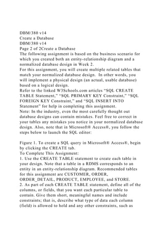
Note: In the industry, even the most carefully thought out database designs can contain mistakes. Feel free to correct in your tables any mistakes you notice in your normalized database design. Also, note that in Microsoft® Access®, you follow the steps below to launch the SQL editor:
Figure 1. To create a SQL query in Microsoft® Access®, begin by clicking the CREATE tab.
To Complete This Assignment:
1. Use the CREATE TABLE statement to create each table in your design. Note that a table in a RDMS corresponds to an entity in an entity-relationship diagram. Recommended tables for this assignment are CUSTOMER, ORDER, ORDER_DETAIL, PRODUCT, EMPLOYEE, and STORE.
2. As part of each CREATE TABLE statement, define all of the columns, or fields, that you want each particular table to contain. Give them short, meaningful names and include constraints; that is, describe what type of data each column (field) is allowed to hold and any other constraints, such as size, range, or uniqueness.
3. Note that any field you marked as a unique identifier in your normalized database design is a key field. Key fields must be described as both UNIQUE and NOT NULL, which means a value must exist for each record and that value must be unique across all records.
4. After you have created all six tables, including relationships between the tables as appropriate (matching the primary key in one table to a foreign key in another table), use the INSERT INTO statement to insert 10 records into each of your tables. You will need to make up the data you insert into your tables. For example, to insert one record into the CUSTOMER table, you will need to invent a customer number, a customer name, and so on—one value for each of the fields you defined for the CUSTOMER table—to insert into the table.
5. To ensure that your INSERT INTO statements succeeded in populating your tables, use the SELECT statement described in Ch. 7, “Introduction to Structured Query Language,” in Database Systems: Design, Implementation, and Management.to retrieve the records you inserted. For example, to see all 10 records you inserted into the CUSTOMER table, you might apply the following SQL statement: SELECT * FROM CUSTOMER;
After you have created all six tables and populated ten records in each table, submit to the Assignment Files tab the database containin.
Data AnalysisInstructions of Excel 2016By Yancy Chow.docxwhittemorelucilla
Data Analysis
Instructions of Excel 2016
By Yancy Chow
Data Analysis: House Example
House Data : 50 houses
Two variables: Price (Y) Area (X)
Excel: How to Add-in
Setting Up Excel for Statistical Analysis:
Click on Excel FileOptions
3
Excel: How to Add-in
Then find “Add ins” on the left side and click on it.
After that, click on “Go”.
Then click on “OK”.
Excel: How to Add-in
Then find “Analysis ToolPak” and click on it.
---- Click on “OK”.
Note: if you use Apple computer, the “add-in” option is under “Tool”!
Excel: How to Add-in
Now you’ve successfully added in the “Data Analysis”.
Click on “Data” on the top, now you can see “Data Analysis” icon!
Excel: How to Calculate
Mean, Median and Mode?
Open your data in Excel or type your data in Excel by column. For example, we want to calculate the mean, median and mode for the variable “Price” in this data. Select “Data” firstly, then click on “Data Analysis”
Excel: How to Calculate
Mean, Median and Mode?
After you clicking on “Data Analysis”, scroll the mouse until you find “Descriptive Statistics” in the Analysis Tools Panel and then select it. Then click on “OK”.
Excel: How to Calculate
Mean, Median and Mode?
Firstly, you need to input the “Input Range”.
You can either input by typing in the box or clicking using the mouse to select the data numbers in the column which you are interested in. In this example, we select the all 50 numbers in the first column. Do not select the label row, like “price” row.
9
Excel: How to Calculate
Mean, Median and Mode?
After selecting the “Input Range”, you need to select “Output Range” and choose anywhere you want to the output to be.
Excel: How to Calculate
Mean, Median and Mode?
Then select “Summary statistics”. Click on “OK” and you will have the data analysis results.
Excel: How to Calculate
Mean, Median and Mode?
Here is the results from the data analysis, including the information such like mean, median, mode , standard deviation, sample variance, rang, minimum and maximum.
Note that EXCEL can only find one mode. You need to check whether there is mort than one by your own.
Excel: How to Calculate the
first Quartiles (Q1)?
Q1: Choose an empty space, enter:
“=quartile(data range, 1)”
Then press “Enter” and you will get the first quartile (Q1) result.
A2:A51 is the range of the data
Excel: How to Calculate the
third Quartiles (Q3)?
Q1: Choose an empty space, enter:
“=quartile(data range, 3)”
Then press “Enter” and you will get the third quartile (Q3) result.
A2:A51 is the range of the data
Excel: How to Draw Histograms?
Firstly, check the output from the “Descriptive Statistics” in “Data Analysis”. We notice in this house data, mean is $956396.66, minimum is $729870 and maximum is $1190000. A reasonable will be $50000. So create a new Colum of the “Bins” which is from .
BUS 308 Week 4 Lecture 3 Developing Relationships in Exc.docxShiraPrater50
BUS 308 Week 4 Lecture 3
Developing Relationships in Excel
Expected Outcomes
After reading this lecture, the student should be able to:
1. Calculate the t-value for a correlation coefficient
2. Calculate the minimum statistically significant correlation coefficient value.
3. Set-up and interpret a Linear Regression in Excel
4. Set-up and interpret a Multiple Regression in Excel
Overview
Setting up correlations and regressions in Excel is fairly straightforward and follows the
approaches we have seen with our previous tools. This involves setting up the data input table,
selecting the tools, and inputting information into the appropriate parts of the input window.
Correlations
Question 1
Data set-up for a correlation is perhaps the simplest of any we have seen. It involves
simply copying and pasting the variables from the Data tab to the Week 4 worksheet. Again,
paste them to the right of the question area. The screenshot below has the data for both the
question 1 correlation and the question 2 multiple regression pasted them starting at column V.
You can paste all the data at once or add the multiple regression variables later (as long as you
do not sort the original data).
Specifically, for Question 1, copy the salary data to column V (for example). Then copy
the Midpoint thru Service columns and paste them next to salary. Finally copy the Raise column
and paste it next to the service column. Notice that our data input range for this question now
includes Salary in Column V and the other interval level variables found in Columns W thru AA.
Question 1 asks for the correlation among the interval/ratio level variables with salary
and says to exclude compa-ratio. For our example, we will correlation compa-ratio with the
other interval/ratio level variables with the exclusion of salary. Since compa-ratio equals the
salary divided by the midpoint, it does not seem reasonable to use salary in predicting compa-
ratio or compa-ratio in predicting salary.
Pearson correlations can be performed in two ways within Excel. If we have a single pair
of variables we are interested in, for example compa-ratio and performance rating, we could use
the fx (or Formulas) function CORREL(array1, array2) (note array means the same as range) to
give us the correlation.
However, if we have several variables we want to correlate at the same time, it is more
effective to use the Correlation function found in the Analysis ToolPak in the Data Analysis tab.
Set up of the input data for Correlation is simple. Just ensure that all of the variables to be
correlated are listed together, and only include interval or ratio level data. For our data set, this
would mean we cannot include gender or degree; even though they look like numerical data the 0
and 1 are merely labels as far as correlation is concerned.
In the Correlation data input box shown below, list the entire data range, indicate if your
dat ...
Week 3 Lecture 11
Regression Analysis
Regression analysis is the development of an equation that shows the impact of the
independent variables (the inputs we can generally control) on the output result. While the
mathematical language may sound strange, most of you are quite familiar with regression like
instructions and use them quite regularly.
To make a cake, we take 1 box mix, add 1¼ cups of water, ½ cup of oil, and 3 eggs. All
of this is combined and cooked. The recipe is an example of a regression equation. The output
(or result or dependent variable) is the cake, the inputs (or independent variables) are the inputs
used. Each input is accompanied by a coefficient (AKA weight or amount) that tells us how
“much” of the variable is “used” or weighted into the outcome.
So, in an equation format, this cake recipe might look like:
Y = 1X1 + 1.25X2 + .5X3 + 3X4 where:
Y = cake
X1 = box mix
X2 = cups of water
X3 = cups of oil
X4 = an egg.
Of course, for the cake, the recipe needs to go through the cooking process; while for
other regression equations the outputs need to go through whatever “process” turns the inputs
into the output – this is often called “life.”
Example
With a regression analysis, we can identify what factors influence an outcome. So, with
our Salary issue, the natural question to help us answer our research question of do males and
females get equal pay for equal work would be: what factors influence or explain an individual’s
pay? This is a perfect question for a multi-variate regression. Multi-variate simply means we have
multiple input variables with a single output variable (Lind, Marchel, & Wathen, 2008).
Variables. A regression analysis uses two distinct types of data. The first are variables
that are at least interval level or better (the same as the other techniques we have used so far).
The other is called a dummy variable, a variable that can be coded 0 or 1 indicating the presence
of some characteristic. In our data set, we have two variables that can be used as dummy coded
variables in a regression, Degree and Gender; both coded 0 or 1. In the case of Degree, the 0
stands for having a bachelor’s degree and the 1 stands for having an advanced degree. For
Gender, 0 means a male and 1 means a female. How these are interpreted in a regression output
will be discussed below. For now, the significance of dummy coding is that it allows us to
include nominal or ordinal data in our analysis.
Excel Approach. For our question of what factors influence pay, we will use Excel’s
Regression function found in the Data Analysis section. This function will produce two output
tables of interest. The first table tests to see if the entire regression equation is statistically
significant; that is, do the input variables significantly impact the output variable. If so, we
would then examine the second table – the coefficients used in a regression equation for e.
Using microsoft excel for weibull analysisMelvin Carter
A simple introduction to reliability analysis of components. Though this lacks explanations of the calculated steps it shows how simple analysis can be. Note that it only addresses the Weibull distribution. It does share how to look elsewhere if the Weibull shape parameter is not near the ideal three(3).
Elementary Data Analysis with MS Excel_Day-4Redwan Ferdous
This event took place on 12th September 2020. This was arranged by EMK Center (Makerlab). The title was 'Elementary Data Analysis with MS Excel', where very basic data analysis with MS excel was discussed.
In Day-4, the MS Excel Data Tab, View and Review tab as well as Developer Tab of Horizontal top ribbon was discussed. As well as different Quick analysis tools, What-if Analysis, Data Table, Scenario Manager, Pareto Chart was also discussed.
In this tutorial, we discuss how to do a regression analysis in Excel. I will teach you how to activate the regression analysis feature, what are the functions and methods we can use to do a regression analysis in Excel and most importantly, how to interpret the regression analysis results. Source: https://tinytutes.com/tutorials/regression-analysis-in-excel/
I am Robert M. I am a Quantitative Analysis Homework Expert at excelhomeworkhelp.com. I hold a Master's in Statistics, from Birmingham, United States. I have been helping students with their homework for the past 7 years. I solved homework related to Quantitative Analysis.
Visit excelhomeworkhelp.com or email info@excelhomeworkhelp.com. You can also call on +1 678 648 4277 for any assistance with Quantitative Analysis Homework.
Using Microsoft Excel for Weibull Analysis by William DornerMelvin Carter
I placed the original Quality Digest article (1/1/1999) in Word to clarify the equations used to perform analysis on a data set have Weibull distribution characteristics.
Convenience shoppingSTAT-S301Fall 2019Question Set 1.docxbobbywlane695641
Convenience shopping
STAT-S301
Fall 2019
Question Set 1
1. Get to know your scientific question (Chapter 1)
(a) Identify the variable of interest.
(b) Identify the population(s) and sample(s).
(c) Identify the parameter(s) and statistic(s).
(d) What is the scientific question? Is this Descriptive Statistics or Inferential Statistics?
2. Get to know your data (Chapter 1)
(a) Identify the types of your data: nominal data, ordinal data or quantitative data.
(b) Identify the types of your data: time series data or cross-sectional data.
(c) Identify the source of your data: primary data or secondary data. Do you think the data is
reliable? Are there possible issues with your data?
3. Calculate descriptive statistics in Excel (Chapter 3)
(a) Calculate the statistics for your variable of interest, such as sample mean (x̄), median, mode,
variance (s2), and standard deviation (s).
(b) Identify two different groups based on the qualitative data. Calculate the above statistics for
each group to compare.
4. Display your data with charts and graphs in Excel (Chapter 2)
(a) Construct displays that best describe your qualitative variable (e.g. bar chart, pie chart); and
describe the distribution.
(b) Construct displays that best describe your variable of interest and describe its distribution. (Use:
Frequency distribution tables, histograms and/or the empirical rule to discuss normality, symmetry
and skewness)
(c) Construct displays that best describe the relationship/association between two quantitative
variables (the variable of interest as the dependent variable, y, and another quantitative
variable as the independent variable, x); and describe the relationship.
5. Distributions (Chapters 5-6)
(a) Consider the distribution of your quantitative data in 4(b). Would it be appropriate to use the
Binomial or Normal distribution to model your data? Why or why not? Hint: The binomial
distribution models success/failure discrete data while the normal distribution is for bell-
shaped continuous data.
1
Question Set 2
1. Construct a confidence interval for a population mean (Chapter 8)
(a) Do you need to make assumptions in order to perform the procedure of constructing a
confidence interval? If so, what assumptions need to be made? If not, why?
(b) Construct a confidence interval for the average sales .
i. Should you use a z-interval or a t-interval? Why?
ii. Compute the necessary sample statistics for constructing a confidence interval.
iii. Find the margin of error of the confidence interval at confidence levels of 92% and 95%,
respectively.
iv. Calculate these two confidence intervals.
(c) Someone believes that the average sales is 2421 Dollars. Does the sample support the claim?
Explain if you have different conclusions using the above two confidence intervals. (You must
discuss in terms of accuracy and precision.)
2. Conduct a hypothesis test for a population mean (Chapter 9)
(a) Do you need to make assumptions in order to p.
1. Outline the differences between Hoarding power and Encouraging..docxpaynetawnya
1. Outline the differences between Hoarding power and Encouraging.
2. Explain about the power of Congruency in Leadership.
DataIDSalaryCompaMidpoint AgePerformance RatingServiceGenderRaiseDegreeGender1GrCopy Employee Data set to this page.822.10.962233290915.81FAThe ongoing question that the weekly assignments will focus on is: Are males and females paid the same for equal work (under the Equal Pay Act)? 1522.60.984233280814.91FANote: to simplfy the analysis, we will assume that jobs within each grade comprise equal work.3522.60.984232390415.30FA37230.999232295216.20FAThe column labels in the table mean:1023.11.003233080714.71FAID – Employee sample number Salary – Salary in thousands 2323.11.004233665613.30FAAge – Age in yearsPerformance Rating – Appraisal rating (Employee evaluation score)1123.31.01223411001914.81FASERvice – Years of serviceGender: 0 = male, 1 = female 2623.51.020232295216.20FAMidpoint – salary grade midpoint Raise – percent of last raise3123.61.028232960413.91FAGrade – job/pay gradeDegree (0= BS\BA 1 = MS)3623.61.026232775314.30FAGender1 (Male or Female)Compa-ratio - salary divided by midpoint4023.81.034232490206.30MA14241.04523329012161FA4224.21.0512332100815.71FA1924.31.055233285104.61MA25251.0872341704040MA3226.50.855312595405.60MB227.70.895315280703.90MB3428.60.923312680204.91MB3933.91.094312790615.50FB2034.11.1013144701614.80FB1834.51.1133131801115.60FB335.11.132313075513.61FB1341.11.0274030100214.70FC741.31.0324032100815.71FC1642.21.054404490405.70MC4145.81.144402580504.30MC2746.91.172403580703.91MC548.21.0044836901605.71MD3049.31.0274845901804.30MD2456.31.173483075913.80FD4556.91.185483695815.21FD4757.21.003573795505.51ME3357.51.008573590905.51ME4581.01857421001605.51ME3858.81.0325745951104.50ME5059.61.0465738801204.60ME4660.21.0575739752003.91ME2260.31.257484865613.81FD161.61.081573485805.70ME4461.81.0855745901605.21ME49631.1055741952106.60ME1763.71.1185727553131FE1264.71.1355752952204.50ME4869.51.2195734901115.31FE973.91.103674910010041MF4375.61.1286742952015.50FF2976.31.139675295505.40MF2177.21.1526743951306.31MF678.11.1656736701204.51MF2878.31.169674495914.40FF
Week 2This assignment covers the material presented in weeks 1 and 2.Six QuestionsBefore starting this assignment, make sure the the assignment data from the Employee Salary Data Set file is copied over to this Assignment file.You can do this either by a copy and paste of all the columns or by opening the data file, right clicking on the Data tab, selecting Move or Copy, and copying the entire sheet to this file(Weekly Assignment Sheet or whatever you are calling your master assignment file).It is highly recommended that you copy the data columns (with labels) and paste them to the right so that whatever you do will not disrupt the original data values and relationships.To Ensure full credit for each question, you need to show how you got your results. For example, Question 1 asks for several data values. If you obtain them using descript ...
TOPIC Bench-marking Testing1. Windows operating system (Microso.docxjuliennehar
TOPIC: Bench-marking Testing
1. Windows operating system (Microsoft Windows 10 Pro 10.0.17763) in terms of what the literature says about the efficiencies AND inefficiencies for each in terms of Performance that you will measure (graphics, cpu, memory, file storage). This section should be really detailed and contain subheadings. Basically there are 4 sections.
2. Research what benchmarking is, its purpose, why its a valuable tool for IT managers.
3. Research at least two benchmark tools that you can use in your research (so free and downloadable). 2 for Windows Describe what the benchmark tool is, who developed it, and find a case study where its been used (if possible).
4. Discuss the data and visual reports that the tool will give you so you can compare the results. Be specific here...this is critical to success.
***You need at least 2 references PER fact. You must use APA inline citations.
8. A 2 x 2 Experimental Design: - Quality and Economy (x1 and x2 manipulation checks)
Dr. Boonghee Yoo
[email protected]
RMI Distinguished Professor in Business and
Professor of Marketing & International Business
Run factor analysis for x1 and x2 manipulation check questions.
2
x1 MC - Perceived service quality
x2 MC - Perceived contribution to local economy
Compute the composite variable for each x MC.
3
Create x1MC and x2MC.
Run t-test to check if the manipulation is well done.
Test variable (x1MC here):
Interval- or ratio-scaled
variable(s)
Grouping variable (x1 here):
A nominal-scaled variable:
Select two groups that
you want to compare.
Independent-samples t-test
Step 1.
See the sample mean of each group.
See if the mean difference is as expected (e.g., Hi > Low).
Step 2. Levene’s test (Ho: s2group1 = s2group2)
If p-value of Levene’s test > alpha, read the “Equal variances assumed” line.
If p-value < alpha, read the “Equal variances NOT assumed” line.
Step 3. t-test
Read the t-value, which is the test statistics.
And read p-value.
Levene’s test (Ho: s2group1 = s2group2)
The graph confirms a successful manipulation.
6
The service quality of the “High” scenario is perceived to be higher than that of the “Low” scenario.
8. A 2 x 2 Experimental Design: - Quality and Economy (x1 and x2 as independent variables)
Dr. Boonghee Yoo
[email protected]
RMI Distinguished Professor in Business and
Professor of Marketing & International Business
Make changes on the names, labels, and measure on the variable view.
Check the measure.
Have the same keys between “Name” and “Label.”
Run factor analysis for ys (dependent variables).
Select “Principal axis factoring” from “Extraction.”
The two-factor solution seems the best as (1) they are over one eigenvalue each and (2) the variance explained for is over 60%.
The new eigenvalues after the rotation.
The rotated factor matrix is clear.
But note that y3 and y1 are collapsed into one factor.
If ...
Excel Files AssingmentsCopy of Student_Assignment_File.11.01..docxSANSKAR20
Excel Files Assingments/Copy of Student_Assignment_File.11.01.2016.xlsx
DataIDSalaryCompa-ratioMidpointAgePerformance RatingServiceGenderRaiseDegreeGender1GradeCopy Employee Data set to this page.The ongoing question that the weekly assignments will focus on is: Are males and females paid the same for equal work (under the Equal Pay Act)? Note: to simplfy the analysis, we will assume that jobs within each grade comprise equal work.The column labels in the table mean:ID – Employee sample number Salary – Salary in thousands Age – Age in yearsPerformance Rating – Appraisal rating (Employee evaluation score)SERvice – Years of serviceGender: 0 = male, 1 = female Midpoint – salary grade midpoint Raise – percent of last raiseGrade – job/pay gradeDegree (0= BS\BA 1 = MS)Gender1 (Male or Female)Compa-ratio - salary divided by midpoint
Week 2This assignment covers the material presented in weeks 1 and 2.Six QuestionsBefore starting this assignment, make sure the the assignment data from the Employee Salary Data Set file is copied over to this Assignment file.You can do this either by a copy and paste of all the columns or by opening the data file, right clicking on the Data tab, selecting Move or Copy, and copying the entire sheet to this file(Weekly Assignment Sheet or whatever you are calling your master assignment file).It is highly recommended that you copy the data columns (with labels) and paste them to the right so that whatever you do will not disrupt the original data values and relationships.To Ensure full credit for each question, you need to show how you got your results. For example, Question 1 asks for several data values. If you obtain them using descriptive statistics,then the cells should have an "=XX" formula in them, where XX is the column and row number showing the value in the descriptive statistics table. If you choose to generate each value using fxfunctions, then each function should be located in the cell and the location of the data values should be shown.So, Cell D31 - as an example - shoud contain something like "=T6" or "=average(T2:T26)". Having only a numerical value will not earn full credit.The reason for this is to allow instructors to provide feedback on Excel tools if the answers are not correct - we need to see how the results were obtained.In starting the analysis on a research question, we focus on overall descriptive statistics and seeing if differences exist. Probing into reasons and mitigating factors is a follow-up activity.1The first step in analyzing data sets is to find some summary descriptive statistics for key variables. Since the assignment problems willfocus mostly on the compa-ratios, we need to find the mean, standard deviations, and range for our groups: Males, Females, and Overall.Sorting the compa-ratios into male and females will require you copy and paste the Compa-ratio and Gender1 columns, and then sort on Gender1.The values for age, performance rating, and service are prov ...
Week 4 Lecture 12 Significance Earlier we discussed co.docxcockekeshia
Week 4 Lecture 12
Significance
Earlier we discussed correlations without going into how we can identify statistically
significant values. Our approach to this uses the t-test. Unfortunately, Excel does not
automatically produce this form of the t-test, but setting it up within an Excel cell is fairly easy.
And, with some slight algebra, we can determine the minimum value that is statistically
significant for any table of correlations all of which have the same number of pairs (for example,
a Correlation table for our data set would use 50 pairs of values, since we have 50 members in
our sample).
The t-test formula for a correlation (r) is t = r * sqrt(n-2)/sqrt(1-r2); the associated degrees
of freedom are n-2 (number of pairs – 2) (Lind, Marchel, & Wathen, 2008). For some this might
look a bit off-putting, but remember that we can translate this into Excel cells and functions and
have Excel do the arithmetic for us.
Excel Example
If we go back to our correlation table for salary, midpoint, Age, Perf Rat, Service, and
Raise, we have:
Using Excel to create the formula and cell numbers for our key values allows us to
quickly create a result. The T.dist.2t gives us a p-value easily.
The formula to use in finding the minimum correlation value that is statistically
significant is r = sqrt(t^2/(t^2 + n-2)). We would find the appropriate t value by using the
t.inv.2T(alpha, df) with alpha = 0.05 and df = n-2 or 48. Plugging these values into the gives us
a t-value of 2.0106 or 2.011(rounded).
Putting 2.011 and 48 (n-2) into our formula gives us a r value of 0.278; therefore, in a
correlation table based on 50 pairs, any correlation greater or equal to 0.278 would be
statistically significant.
Technical Point. If you are interested in how we obtained the formula for determining
the minimum r value, the approach is shown below. If you are not interested in the math, you
can safely skip this paragraph.
t = r* sqrt(n-2)/sqrt(1-r2)
Multiplying gives us t *sqrt (1- r2) = r2* (n-2)
Squaring gives us: t2 * (1- r2) = r2* (n-2)
Multiplying out gives us: t2– t2* r2 = n r2-2* r2
Adding gives us: t2= n* r2-2*r2+ t2 *r2
Factoring gives us t2= r2 *(n -2+ t2)
Dividing gives us t2 / (n -2+ t2) = r2
Taking the square root gives us r = sqrt (t2 / (n -2+ t2)
Effect Size Measures
As we have discussed, there is a difference between statistical and practical
significance. Virtually any statistic can become statistically significant if the sample is large
enough. In practical terms, a correlation of .30 and below is generally considered too weak to be
of any practical significance. Additionally, the effect size measure for Pearson’s correlation is
simply the absolute value of the correlation; the outcome has the same general interpretation as
Cohen’s D for the t-test (0.8 is strong, and 0.2 is quite weak, for example) (Tanner & Youssef-
Morgan, 2013).
Spearman’s Rank Correlation
Another typ.
Deadline 6 PM Friday September 27, 201310 Project Management Que.docxedwardmarivel
Deadline 6 PM Friday September 27, 2013
10 Project Management Questions with sub-questions under each question. A word document is provided with all questions and directions.
Problem 1
The following data were obtained from a project to create a new portable electronic.
Activity
Duration
Predecessors
A
5 Days
---
B
6 Days
---
C
8 Days
---
D
4 Days
A, B
E
3 Days
C
F
5 Days
D
G
5 Days
E, F
H
9 Days
D
I
12 Days
G
Step 1: Construct a network diagram for the project.
Step 2: Answer the following questions:
a)
What is the Scheduled Completion of the Project?
b)
What is the Critical Path of the Project?
c)
What is the ES for Activity D?
d)
What is the LS for Activity G?
e)
What is the EF for Activity B?
f)
What is the LF for Activity H?
g)
What is the float for Activity I?
Problem 2
The following data were obtained from a project to build a pressure vessel:
Activity
Duration
Predecessors
A
6 weeks
---
B
6 weeks
---
C
5 weeks
B
D
4 weeks
A, C
E
5 weeks
B
F
7 weeks
D, E, G
G
4 weeks
B
H
8 weeks
F
I
5 weeks
G
J
3 week
I
Step 1: Construct a network diagram for the project.
Step 2: Answer the following questions:
a)
Calculate the scheduled completion time.
b)
Identify the critical path
c)
What is the slack time (float) for activity A?
d)
What is the slack time (float) for activity D?
e) What is the slack time (float) for activity E?
f) What is the slack time (float) for activity G?
Problem 3
The following data were obtained from a project to design a new software package:
Activity
Duration
Predecessors
A
5 Days
---
B
8 Days
---
C
6 Days
A
D
4 Days
C, B
E
5 Days
A
F
4 Days
D, E, G
G
4 Days
B, C
H
3 Day
G
Step 1: Construct a network diagram for the project.
Step 2: Answer the following questions:
a)
Calculate the scheduled completion time.
b)
Identify the critical path(s)
c)
What is the slack time (float) for activity B?
d)
What is the slack time (float) for activity D?
e) What is the slack time (float) for activity E?
f) What is the slack time (float) for activity G?
Problem 4
The following data were obtained from an in-house MIS project:
Activity
Duration
Predecessors
A
5 Days
---
B
8 Days
---
C
5 Days
A
D
4 Days
B
E
5 Days
B
F
3 Day
C, D
G
7 Days
C, D
H
6 Days
E, F, G
I
9 Days
E, F
Step 1: Construct a network diagram for the project.
Step 2: Answer the following questions:
a)
Calculate the scheduled completion time.
b)
Identify the critical path
c)
What is the slack time (float) for activity A?
d)
What is the slack time (float) for activity D?
e)
What is the slack time (float) for activity E?
f)
What is the slack time (float) for activity F?
PROBLEM 5
Use the network diagram below and the additional information provided to answer the corresponding questions.
a) Give the crash cost per day per activity.
b) Which activities should be crash.
More Related Content
Similar to DBM380 v14Create a DatabaseDBM380 v14Page 2 of 2Create a D.docx
Elementary Data Analysis with MS Excel_Day-4Redwan Ferdous
This event took place on 12th September 2020. This was arranged by EMK Center (Makerlab). The title was 'Elementary Data Analysis with MS Excel', where very basic data analysis with MS excel was discussed.
In Day-4, the MS Excel Data Tab, View and Review tab as well as Developer Tab of Horizontal top ribbon was discussed. As well as different Quick analysis tools, What-if Analysis, Data Table, Scenario Manager, Pareto Chart was also discussed.
In this tutorial, we discuss how to do a regression analysis in Excel. I will teach you how to activate the regression analysis feature, what are the functions and methods we can use to do a regression analysis in Excel and most importantly, how to interpret the regression analysis results. Source: https://tinytutes.com/tutorials/regression-analysis-in-excel/
I am Robert M. I am a Quantitative Analysis Homework Expert at excelhomeworkhelp.com. I hold a Master's in Statistics, from Birmingham, United States. I have been helping students with their homework for the past 7 years. I solved homework related to Quantitative Analysis.
Visit excelhomeworkhelp.com or email info@excelhomeworkhelp.com. You can also call on +1 678 648 4277 for any assistance with Quantitative Analysis Homework.
Using Microsoft Excel for Weibull Analysis by William DornerMelvin Carter
I placed the original Quality Digest article (1/1/1999) in Word to clarify the equations used to perform analysis on a data set have Weibull distribution characteristics.
Convenience shoppingSTAT-S301Fall 2019Question Set 1.docxbobbywlane695641
Convenience shopping
STAT-S301
Fall 2019
Question Set 1
1. Get to know your scientific question (Chapter 1)
(a) Identify the variable of interest.
(b) Identify the population(s) and sample(s).
(c) Identify the parameter(s) and statistic(s).
(d) What is the scientific question? Is this Descriptive Statistics or Inferential Statistics?
2. Get to know your data (Chapter 1)
(a) Identify the types of your data: nominal data, ordinal data or quantitative data.
(b) Identify the types of your data: time series data or cross-sectional data.
(c) Identify the source of your data: primary data or secondary data. Do you think the data is
reliable? Are there possible issues with your data?
3. Calculate descriptive statistics in Excel (Chapter 3)
(a) Calculate the statistics for your variable of interest, such as sample mean (x̄), median, mode,
variance (s2), and standard deviation (s).
(b) Identify two different groups based on the qualitative data. Calculate the above statistics for
each group to compare.
4. Display your data with charts and graphs in Excel (Chapter 2)
(a) Construct displays that best describe your qualitative variable (e.g. bar chart, pie chart); and
describe the distribution.
(b) Construct displays that best describe your variable of interest and describe its distribution. (Use:
Frequency distribution tables, histograms and/or the empirical rule to discuss normality, symmetry
and skewness)
(c) Construct displays that best describe the relationship/association between two quantitative
variables (the variable of interest as the dependent variable, y, and another quantitative
variable as the independent variable, x); and describe the relationship.
5. Distributions (Chapters 5-6)
(a) Consider the distribution of your quantitative data in 4(b). Would it be appropriate to use the
Binomial or Normal distribution to model your data? Why or why not? Hint: The binomial
distribution models success/failure discrete data while the normal distribution is for bell-
shaped continuous data.
1
Question Set 2
1. Construct a confidence interval for a population mean (Chapter 8)
(a) Do you need to make assumptions in order to perform the procedure of constructing a
confidence interval? If so, what assumptions need to be made? If not, why?
(b) Construct a confidence interval for the average sales .
i. Should you use a z-interval or a t-interval? Why?
ii. Compute the necessary sample statistics for constructing a confidence interval.
iii. Find the margin of error of the confidence interval at confidence levels of 92% and 95%,
respectively.
iv. Calculate these two confidence intervals.
(c) Someone believes that the average sales is 2421 Dollars. Does the sample support the claim?
Explain if you have different conclusions using the above two confidence intervals. (You must
discuss in terms of accuracy and precision.)
2. Conduct a hypothesis test for a population mean (Chapter 9)
(a) Do you need to make assumptions in order to p.
1. Outline the differences between Hoarding power and Encouraging..docxpaynetawnya
1. Outline the differences between Hoarding power and Encouraging.
2. Explain about the power of Congruency in Leadership.
DataIDSalaryCompaMidpoint AgePerformance RatingServiceGenderRaiseDegreeGender1GrCopy Employee Data set to this page.822.10.962233290915.81FAThe ongoing question that the weekly assignments will focus on is: Are males and females paid the same for equal work (under the Equal Pay Act)? 1522.60.984233280814.91FANote: to simplfy the analysis, we will assume that jobs within each grade comprise equal work.3522.60.984232390415.30FA37230.999232295216.20FAThe column labels in the table mean:1023.11.003233080714.71FAID – Employee sample number Salary – Salary in thousands 2323.11.004233665613.30FAAge – Age in yearsPerformance Rating – Appraisal rating (Employee evaluation score)1123.31.01223411001914.81FASERvice – Years of serviceGender: 0 = male, 1 = female 2623.51.020232295216.20FAMidpoint – salary grade midpoint Raise – percent of last raise3123.61.028232960413.91FAGrade – job/pay gradeDegree (0= BS\BA 1 = MS)3623.61.026232775314.30FAGender1 (Male or Female)Compa-ratio - salary divided by midpoint4023.81.034232490206.30MA14241.04523329012161FA4224.21.0512332100815.71FA1924.31.055233285104.61MA25251.0872341704040MA3226.50.855312595405.60MB227.70.895315280703.90MB3428.60.923312680204.91MB3933.91.094312790615.50FB2034.11.1013144701614.80FB1834.51.1133131801115.60FB335.11.132313075513.61FB1341.11.0274030100214.70FC741.31.0324032100815.71FC1642.21.054404490405.70MC4145.81.144402580504.30MC2746.91.172403580703.91MC548.21.0044836901605.71MD3049.31.0274845901804.30MD2456.31.173483075913.80FD4556.91.185483695815.21FD4757.21.003573795505.51ME3357.51.008573590905.51ME4581.01857421001605.51ME3858.81.0325745951104.50ME5059.61.0465738801204.60ME4660.21.0575739752003.91ME2260.31.257484865613.81FD161.61.081573485805.70ME4461.81.0855745901605.21ME49631.1055741952106.60ME1763.71.1185727553131FE1264.71.1355752952204.50ME4869.51.2195734901115.31FE973.91.103674910010041MF4375.61.1286742952015.50FF2976.31.139675295505.40MF2177.21.1526743951306.31MF678.11.1656736701204.51MF2878.31.169674495914.40FF
Week 2This assignment covers the material presented in weeks 1 and 2.Six QuestionsBefore starting this assignment, make sure the the assignment data from the Employee Salary Data Set file is copied over to this Assignment file.You can do this either by a copy and paste of all the columns or by opening the data file, right clicking on the Data tab, selecting Move or Copy, and copying the entire sheet to this file(Weekly Assignment Sheet or whatever you are calling your master assignment file).It is highly recommended that you copy the data columns (with labels) and paste them to the right so that whatever you do will not disrupt the original data values and relationships.To Ensure full credit for each question, you need to show how you got your results. For example, Question 1 asks for several data values. If you obtain them using descript ...
TOPIC Bench-marking Testing1. Windows operating system (Microso.docxjuliennehar
TOPIC: Bench-marking Testing
1. Windows operating system (Microsoft Windows 10 Pro 10.0.17763) in terms of what the literature says about the efficiencies AND inefficiencies for each in terms of Performance that you will measure (graphics, cpu, memory, file storage). This section should be really detailed and contain subheadings. Basically there are 4 sections.
2. Research what benchmarking is, its purpose, why its a valuable tool for IT managers.
3. Research at least two benchmark tools that you can use in your research (so free and downloadable). 2 for Windows Describe what the benchmark tool is, who developed it, and find a case study where its been used (if possible).
4. Discuss the data and visual reports that the tool will give you so you can compare the results. Be specific here...this is critical to success.
***You need at least 2 references PER fact. You must use APA inline citations.
8. A 2 x 2 Experimental Design: - Quality and Economy (x1 and x2 manipulation checks)
Dr. Boonghee Yoo
[email protected]
RMI Distinguished Professor in Business and
Professor of Marketing & International Business
Run factor analysis for x1 and x2 manipulation check questions.
2
x1 MC - Perceived service quality
x2 MC - Perceived contribution to local economy
Compute the composite variable for each x MC.
3
Create x1MC and x2MC.
Run t-test to check if the manipulation is well done.
Test variable (x1MC here):
Interval- or ratio-scaled
variable(s)
Grouping variable (x1 here):
A nominal-scaled variable:
Select two groups that
you want to compare.
Independent-samples t-test
Step 1.
See the sample mean of each group.
See if the mean difference is as expected (e.g., Hi > Low).
Step 2. Levene’s test (Ho: s2group1 = s2group2)
If p-value of Levene’s test > alpha, read the “Equal variances assumed” line.
If p-value < alpha, read the “Equal variances NOT assumed” line.
Step 3. t-test
Read the t-value, which is the test statistics.
And read p-value.
Levene’s test (Ho: s2group1 = s2group2)
The graph confirms a successful manipulation.
6
The service quality of the “High” scenario is perceived to be higher than that of the “Low” scenario.
8. A 2 x 2 Experimental Design: - Quality and Economy (x1 and x2 as independent variables)
Dr. Boonghee Yoo
[email protected]
RMI Distinguished Professor in Business and
Professor of Marketing & International Business
Make changes on the names, labels, and measure on the variable view.
Check the measure.
Have the same keys between “Name” and “Label.”
Run factor analysis for ys (dependent variables).
Select “Principal axis factoring” from “Extraction.”
The two-factor solution seems the best as (1) they are over one eigenvalue each and (2) the variance explained for is over 60%.
The new eigenvalues after the rotation.
The rotated factor matrix is clear.
But note that y3 and y1 are collapsed into one factor.
If ...
Excel Files AssingmentsCopy of Student_Assignment_File.11.01..docxSANSKAR20
Excel Files Assingments/Copy of Student_Assignment_File.11.01.2016.xlsx
DataIDSalaryCompa-ratioMidpointAgePerformance RatingServiceGenderRaiseDegreeGender1GradeCopy Employee Data set to this page.The ongoing question that the weekly assignments will focus on is: Are males and females paid the same for equal work (under the Equal Pay Act)? Note: to simplfy the analysis, we will assume that jobs within each grade comprise equal work.The column labels in the table mean:ID – Employee sample number Salary – Salary in thousands Age – Age in yearsPerformance Rating – Appraisal rating (Employee evaluation score)SERvice – Years of serviceGender: 0 = male, 1 = female Midpoint – salary grade midpoint Raise – percent of last raiseGrade – job/pay gradeDegree (0= BS\BA 1 = MS)Gender1 (Male or Female)Compa-ratio - salary divided by midpoint
Week 2This assignment covers the material presented in weeks 1 and 2.Six QuestionsBefore starting this assignment, make sure the the assignment data from the Employee Salary Data Set file is copied over to this Assignment file.You can do this either by a copy and paste of all the columns or by opening the data file, right clicking on the Data tab, selecting Move or Copy, and copying the entire sheet to this file(Weekly Assignment Sheet or whatever you are calling your master assignment file).It is highly recommended that you copy the data columns (with labels) and paste them to the right so that whatever you do will not disrupt the original data values and relationships.To Ensure full credit for each question, you need to show how you got your results. For example, Question 1 asks for several data values. If you obtain them using descriptive statistics,then the cells should have an "=XX" formula in them, where XX is the column and row number showing the value in the descriptive statistics table. If you choose to generate each value using fxfunctions, then each function should be located in the cell and the location of the data values should be shown.So, Cell D31 - as an example - shoud contain something like "=T6" or "=average(T2:T26)". Having only a numerical value will not earn full credit.The reason for this is to allow instructors to provide feedback on Excel tools if the answers are not correct - we need to see how the results were obtained.In starting the analysis on a research question, we focus on overall descriptive statistics and seeing if differences exist. Probing into reasons and mitigating factors is a follow-up activity.1The first step in analyzing data sets is to find some summary descriptive statistics for key variables. Since the assignment problems willfocus mostly on the compa-ratios, we need to find the mean, standard deviations, and range for our groups: Males, Females, and Overall.Sorting the compa-ratios into male and females will require you copy and paste the Compa-ratio and Gender1 columns, and then sort on Gender1.The values for age, performance rating, and service are prov ...
Week 4 Lecture 12 Significance Earlier we discussed co.docxcockekeshia
Week 4 Lecture 12
Significance
Earlier we discussed correlations without going into how we can identify statistically
significant values. Our approach to this uses the t-test. Unfortunately, Excel does not
automatically produce this form of the t-test, but setting it up within an Excel cell is fairly easy.
And, with some slight algebra, we can determine the minimum value that is statistically
significant for any table of correlations all of which have the same number of pairs (for example,
a Correlation table for our data set would use 50 pairs of values, since we have 50 members in
our sample).
The t-test formula for a correlation (r) is t = r * sqrt(n-2)/sqrt(1-r2); the associated degrees
of freedom are n-2 (number of pairs – 2) (Lind, Marchel, & Wathen, 2008). For some this might
look a bit off-putting, but remember that we can translate this into Excel cells and functions and
have Excel do the arithmetic for us.
Excel Example
If we go back to our correlation table for salary, midpoint, Age, Perf Rat, Service, and
Raise, we have:
Using Excel to create the formula and cell numbers for our key values allows us to
quickly create a result. The T.dist.2t gives us a p-value easily.
The formula to use in finding the minimum correlation value that is statistically
significant is r = sqrt(t^2/(t^2 + n-2)). We would find the appropriate t value by using the
t.inv.2T(alpha, df) with alpha = 0.05 and df = n-2 or 48. Plugging these values into the gives us
a t-value of 2.0106 or 2.011(rounded).
Putting 2.011 and 48 (n-2) into our formula gives us a r value of 0.278; therefore, in a
correlation table based on 50 pairs, any correlation greater or equal to 0.278 would be
statistically significant.
Technical Point. If you are interested in how we obtained the formula for determining
the minimum r value, the approach is shown below. If you are not interested in the math, you
can safely skip this paragraph.
t = r* sqrt(n-2)/sqrt(1-r2)
Multiplying gives us t *sqrt (1- r2) = r2* (n-2)
Squaring gives us: t2 * (1- r2) = r2* (n-2)
Multiplying out gives us: t2– t2* r2 = n r2-2* r2
Adding gives us: t2= n* r2-2*r2+ t2 *r2
Factoring gives us t2= r2 *(n -2+ t2)
Dividing gives us t2 / (n -2+ t2) = r2
Taking the square root gives us r = sqrt (t2 / (n -2+ t2)
Effect Size Measures
As we have discussed, there is a difference between statistical and practical
significance. Virtually any statistic can become statistically significant if the sample is large
enough. In practical terms, a correlation of .30 and below is generally considered too weak to be
of any practical significance. Additionally, the effect size measure for Pearson’s correlation is
simply the absolute value of the correlation; the outcome has the same general interpretation as
Cohen’s D for the t-test (0.8 is strong, and 0.2 is quite weak, for example) (Tanner & Youssef-
Morgan, 2013).
Spearman’s Rank Correlation
Another typ.
Similar to DBM380 v14Create a DatabaseDBM380 v14Page 2 of 2Create a D.docx (20)
Deadline 6 PM Friday September 27, 201310 Project Management Que.docxedwardmarivel
Deadline 6 PM Friday September 27, 2013
10 Project Management Questions with sub-questions under each question. A word document is provided with all questions and directions.
Problem 1
The following data were obtained from a project to create a new portable electronic.
Activity
Duration
Predecessors
A
5 Days
---
B
6 Days
---
C
8 Days
---
D
4 Days
A, B
E
3 Days
C
F
5 Days
D
G
5 Days
E, F
H
9 Days
D
I
12 Days
G
Step 1: Construct a network diagram for the project.
Step 2: Answer the following questions:
a)
What is the Scheduled Completion of the Project?
b)
What is the Critical Path of the Project?
c)
What is the ES for Activity D?
d)
What is the LS for Activity G?
e)
What is the EF for Activity B?
f)
What is the LF for Activity H?
g)
What is the float for Activity I?
Problem 2
The following data were obtained from a project to build a pressure vessel:
Activity
Duration
Predecessors
A
6 weeks
---
B
6 weeks
---
C
5 weeks
B
D
4 weeks
A, C
E
5 weeks
B
F
7 weeks
D, E, G
G
4 weeks
B
H
8 weeks
F
I
5 weeks
G
J
3 week
I
Step 1: Construct a network diagram for the project.
Step 2: Answer the following questions:
a)
Calculate the scheduled completion time.
b)
Identify the critical path
c)
What is the slack time (float) for activity A?
d)
What is the slack time (float) for activity D?
e) What is the slack time (float) for activity E?
f) What is the slack time (float) for activity G?
Problem 3
The following data were obtained from a project to design a new software package:
Activity
Duration
Predecessors
A
5 Days
---
B
8 Days
---
C
6 Days
A
D
4 Days
C, B
E
5 Days
A
F
4 Days
D, E, G
G
4 Days
B, C
H
3 Day
G
Step 1: Construct a network diagram for the project.
Step 2: Answer the following questions:
a)
Calculate the scheduled completion time.
b)
Identify the critical path(s)
c)
What is the slack time (float) for activity B?
d)
What is the slack time (float) for activity D?
e) What is the slack time (float) for activity E?
f) What is the slack time (float) for activity G?
Problem 4
The following data were obtained from an in-house MIS project:
Activity
Duration
Predecessors
A
5 Days
---
B
8 Days
---
C
5 Days
A
D
4 Days
B
E
5 Days
B
F
3 Day
C, D
G
7 Days
C, D
H
6 Days
E, F, G
I
9 Days
E, F
Step 1: Construct a network diagram for the project.
Step 2: Answer the following questions:
a)
Calculate the scheduled completion time.
b)
Identify the critical path
c)
What is the slack time (float) for activity A?
d)
What is the slack time (float) for activity D?
e)
What is the slack time (float) for activity E?
f)
What is the slack time (float) for activity F?
PROBLEM 5
Use the network diagram below and the additional information provided to answer the corresponding questions.
a) Give the crash cost per day per activity.
b) Which activities should be crash.
DEADLINE 15 HOURS
6 PAGES
UNDERGRADUATE
COURSEWORK
HARVARD FORMATING
DOUBLE SPACING
INSTRUCTIONS
This assignment seeks to assess your ability to:
• Critically evaluate and discuss the major developments during 2017 in corporate taxation from the perspective of multinational companies and their auditors, governments and other stakeholders.
• Apply appropriate knowledge, analytical techniques and concepts to problems and issues arising from both familiar and unfamiliar situations;
• Think critically, examine problems and issues from a number of perspectives, challenge viewpoints, ideas and concepts and make well-reasoned judgements;
• Present, discuss and defend ideas, concepts and views effectively through formal language.
Background:
In the final weeks of 2017 a leading tax expert suggested that “a whirlwind of international tax changes has swept the globe”. He also went on to say that for companies operating in Europe there is no end in sight to the pace of change. The final recommendations on base erosion and profit shifting (BEPS) from the OECD have been endorsed by the EU. In fact a number of European governments have already implemented large parts of these proposals ahead of schedule.
The third quarter of the year saw the European Commission in the spotlight with its landmark decision that the technology giant Apple must repay no less than €13 billion of taxes to the Irish government. This ruling was based on the view that the favourable tax treatment was effectively state aid and hence the Irish government had broken EU law. At the same time countries across the world continue to compete by reducing the rate of corporate taxes. Many commentators suggest that the UK government will cut the corporate tax rate to 10% if the country fails to negotiate a trade deal with the European Union as part of the Brexit process. In a separate development earlier in the year the government of Hungary announced it would become the tax haven of Central Europe with a plan to reduce corporation tax to a mere 9%.
Required:
You are to write a report for the Board of Directors of a listed global company that has manufacturing and R&D activities across Europe, Asia, Australasia and America. The report should assume that the directors have detailed knowledge of the group activities but are not taxation specialists. However they would be aware of issues relating to corporate governance, transparency and reputational risks.
The report should cover the following aspects:
Evaluate the major developments that occurred in corporate taxation in 2017 and the issues that may arise in the current year.
Discuss the implications for the group in regard to the relationship with its auditors.
Consider how other stakeholders and non-governmental organisations (NGOs) may be affected by changes in the level of corporate taxes and their possible reaction.
The resources below are on Blackboard and provide an introduction to the topic.
“Corpor.
De nada.El gusto es mío.Encantada.Me llamo Pepe.Muy bien, grac.docxedwardmarivel
De nada. El gusto es mío. Encantada. Me llamo Pepe.
Muy bien, gracias. Nada. Nos vemos. Soy de Argentina.
1. ¿Cómo te llamas?
2. ¿Qué hay de nuevo?
3. ¿De dónde eres?
4. Adiós.
5. ¿Cómo está usted?
6. Mucho gusto.
7. Te presento a la señora Díaz.
8. Muchas gracias.
Modelo ¡Hola! Buenos días.
Adiós cómo Chau de eres
es está gusto Hasta Le
mío Muy Soy usted vemos
1. ANA Buenos días, señor González. ¿Cómo (1) (2) ?
SR. GONZÁLEZ (3) bien, gracias. Y tú, ¿(4) estás?
ANA Regular. (5) presento a Antonio.
SR. GONZÁLEZ Mucho (6) , Antonio.
ANTONIO El gusto (7) (8) .
SR. GONZÁLEZ ¿De dónde (9) , Antonio?
ANTONIO (10) (11) México.
ANA (12) luego, señor González.
SR. GONZÁLEZ Nos (13) , Ana.
ANTONIO (14) , señor González.
• • Hasta mañana.
• Nos vemos.
• Buenos días.
• Hasta pronto.
• • ¿Qué tal?
• Regular.
• ¿Qué pasa?
• ¿Cómo estás?
• • Puerto Rico
• Washington
• México
• Estados Unidos
• • Muchas gracias.
• Muy bien, gracias.
• No muy bien.
• Regular.
• • ¿De dónde eres?
• ¿Cómo está usted?
• ¿De dónde es usted?
• ¿Cómo se llama usted?
• • Chau.
• Buenos días.
• Hola.
• ¿Qué tal?
Modelo un papel
unos papeles
1. : unas fotografías
2. : un día
3. : un cuaderno
4. : unos pasajeros
5. : una computadora
6. : unas escuelas
7. : unos videos
8. : un programa
9. : unos autobuses
10. : una palabra
Modelo el señor Díaz
Addresing him: usted
Talking about him: él
1. Don Francisco
Addressing him:
Talking about him:
2. Jimena y Marissa
Addressing them:
Talking about them:
3. Maru y Miguel
Addressing them:
Talking about them:
4. la profesora
Addressing her:
Talking about her:
5. un estudiante
Addressing him:
Talking about him:
6. el director de una escuela
Addressing him:
Talking about him:
7. tres chicas
Addressing them:
Talking about them:
8. un pasajero de autobús
Addressing him:
Talking about him:
9. Juan Carlos y Felipe
Addressing them:
Talking about them:
10. una turista
Addressing her:
Talking about her:
Modelo Ustedes son profesores.
Nosotros somos profesores.
1. Nosotros somos estudiantes.
Ustedes .
2. Usted es de Puerto Rico.
Ella .
3. Nosotros somos conductores.
Ellos .
4. Yo soy turista.
Tú .
5. Ustedes son de México.
Nosotras .
6. Ella es profesora.
Yo .
7. Tú eres de España.
Él .
8. Ellos son pasajeros.
Ellas
Modelo Yo soy Jorge.
1. Hola, me llamo Jorge y de Cuba. Pilar y Nati de España. Pedro, Juan y Paco de México. Todos estudiantes. La señorita Blasco de San Antonio. Ella la profesora. Luis el conductor. Él de Puerto Rico. Ellos de los Estados Unidos. El autobús de la agencia Marazul. Todos pasajeros de la agencia de viajes Marazul. Perdón, ¿de dónde tú, quién ella y de quién las maletas?
Modelo nombre / el pasajero
Es el nombre del pasajero.
.
DDL 24 hours reading the article and writing a 1-page doubl.docxedwardmarivel
DDL:
24 hours
reading the article and writing a
1-page double space
annotated bibliography
including:
1.reference
2.specify the concept you will use
3.explain its significance to the course
4.specify how you'll use it in your project
see the article and project inf below
.
*
DCF valuation methodSuper-normal growth modelApplications: single CF, annuity, perpetuity, uneven CFs, bond, stock, etc.
LECTURE 2 Valuation Basics
(Chapters 4, 6, 7)
*
Amount of cash flows expectedRisk of the cash flows Timing of the cash flow stream
Factors that Determine Value
*
DCF Method: General Formula
Finding PVs is discounting. The discount factor i is determined by the cost of capital invested.
*
10%
Single Cash Flow
100
0
1
2
3
PV = ?
What’s the PV of $100 due in 3 years if i = 10%?
*
Financial Calculator Setup
BGN END
P/Y 1
FORMAT: DEC 4 or larger
*
Financial Calculator
Solution
s
N I/YR PV PMTFV
?
N = 3, I/YR = 10, PMT = 0, FV = 100
CPT, PV
-75.13
/
INPUTS
OUTPUT
*
Spreadsheet
.
DDBA 8307 Week 2 Assignment Exemplar
John Doe[footnoteRef:1] [1: Type your name here]
DDBA 8307-6[footnoteRef:2] [2: Type in DDBA section number (e.g. DDBA 8307 – 6) ]
Dr. Jane Doe[footnoteRef:3] [3: Enter faculty name here.]
1
Scales of Measurement
Type text here. Discuss the implications of “scales of measurement” in quantitative research. Be sure to use a minimum of two citations to support your position(s). Be sure to review the “Scales of Measurement” media from Week 1. This section should be no more than two paragraphs.
Research Question
What are the means, standard deviations, frequencies, and percentages of the Lesson 21 Exercise File variables?
Presentation of Findings
I analyzed data from Lesson 21 Exercise File [footnoteRef:4]. In this section, I present descriptive statistics for the study quantitative and qualitative variables. Appropriate APA tables and figures accompany the analysis[footnoteRef:5]. [4: Insert the appropriate file name. ] [5: The tables and figures from your SPSS output will need to be copied and pasted in the appropriate location.]
Descriptive Statistics[footnoteRef:6] [6: Detailed information can be found in Lesson 20, “Univariate Descriptive Statistics for Qualitative Variables,” and Lesson 21, “Univariate Descriptive Statistics for Quantitative Variables,” in the Green and Salkind text.
]
Descriptive statistics were run for the quantitative and qualitative variables in the Week 1 Assignment data set. Table 1 depicts the means and standard deviations for the quantitative data. Figure 1 depicts a histogram for the GPA variable. Table 2 depicts the frequencies and percentages for the qualitative (categorical) data. Figure 2 depicts a pie chart for the ethnic variable. Appendix 1 depicts the SPSS output.
Table 1[footnoteRef:7] [7: This is an example of an APA-formatted descriptive statistics table. Refer to Sections 5.01-5.19, in the APA Manual for detailed information on APA tables. The descriptive statistics table here includes the appropriate information derived from the SPSS output that is to be pasted as an appendix. Do not split tables across pages. Note: The numbers in the SPSS output presented here are fictitious numbers and do not represent correct numbers in the data set you will use for this application.
]
Means (M) and Standard Deviations (SD) for Study
Quantitative Variables (N = 105)
Variable[footnoteRef:8] [8: You would simply add rows to the table to accommodate the variables you have used in the analysis (i.e., variable 3, variable 4, etc.). Hint: Use the Microsoft Word Table feature.
]
M
SD
GPA
2.78
.76
Final
61.48
7.94
Percent
80.34
12.12
Figure 1. Histogram of GPA distribution.
Table 2[footnoteRef:9] [9: Recall from Lesson 20, “Univariate Descriptive Statistics for Qualitative Variables” (Green & Salkind, 2017), frequencies and percentages are reported for qualitative (nominal) variables. Note: Frequency and percentages are the only c.
DB3.1 Mexico corruptionDiscuss the connection between pol.docxedwardmarivel
DB3.1: Mexico corruption
Discuss the connection between politics, corruption, and criminal organizations in Mexico. How would you go about separating these? Give examples and be specific. Support your ideas on why you would do these specific measures.
DB3.2: Collapse of Soviet Union
How has the collapse of the Soviet Union fostered pirate capitalism and organized crime? Be specific with your answer and support your answer. Do you think that if the Soviet Union did not collapse pirate capitalism and organized crime would still flourish? Support your opinion.
300 words per post
.
DB2Pepsi Co and Coke American beverage giants, must adhere to th.docxedwardmarivel
DB2
Pepsi Co and Coke American beverage giants, must adhere to the U.S Foreign Corruption Act wherever their businesses may take them. Both companies expanded their U.S businesses to India with differing initial results. Coke came home (initially) and Pepsi Co prospered.
Do your research and explain the socio-cultural barriers faced by these two companies? What in your view were the reasons which negatively impacted Coke and positively touched Pepsi Co?
WEEK 3:
Interactive
: Select one company other than the 2 mentioned above, and share this company’s experience in the United Arab Emirates. Comment on another learner’s company experience in a different location of the world.
WEEK 4:
Interactive
: Comment on a different learner’s company experience in a totally different location from those completed earlier. Do you feel that cultural training is an essential pre-requisite for expatriates in any host country? Why/Why not?
Remember to use APA referencing in the body of your posting.
.
DB1 What Ive observedHave you ever experienced a self-managed .docxedwardmarivel
DB1: What I've observed
Have you ever experienced a self-managed team? If so, describe it. If not, why do you think your organization has not embraced self managed teams?
DB2: Case Analysis
Review the case study at the end of Chapter 8, Frederick W. Smith - FedEx. Answer the five questions below:
1. How do the standards set by Fred Smith for FedEx teams improve organizational performance?
2. What motivates the members of FedEx to remain highly engaged in their teams?
3. Describe the role FedEx managers play in facilitating team effectiveness.
4. What types of teams does FedEx use? Provide evidence from the case to support your answer.
5. Leaders play a critical role in building effective teams. Cite evidence from the case that FedEx managers performed some of these roles in developing effective teams.
Image Source Team:
http://www.freedigitalphotos.net/images/gallery-thumbnails.php?id=50143103253525199427035558
.
DB Response 1I agree with the decision to search the house. Ther.docxedwardmarivel
DB Response 1
I agree with the decision to search the house. There was reasonable suspicion to believe the fugitive could have been in the home. The homeowner not only consented to the search of the house but requested it for her safety. Complacency kills. In this situation, the officer is very regretful in his decision to conduct a complacent search of the home, and luckily nobody was killed.
My department does not have body cameras, but I still conduct business as if somebody is recording me. We live in a generation of surveillance. You never know when there are hidden cameras, a camera on a business you did not notice, or a cell phone recording from the top floor of a building. We hire police officers with high amounts of integrity because the definition of integrity is doing the right thing even when nobody is looking. I would be lying if I said my grandmother would approve of everything I do on the job. I am most guilty of foul language and it is something that I am working on not doing that. However, I can emphatically say I work with integrity and honesty without a doubt.
I think setting limits on tolerable behavior in regards to sexual and general harassment is appropriate; however, there are too many situations to make a policy for every behavior one could find inappropriate. When it comes to using force again every situation is different but there should be a pretty well laid out policy at departments for when and how an officer should use a certain amount of force. Officers should be trained on de-escalation tactics and alternatives to using force. Tactical training should include strategies to create time, space, and distance, to reduce the likelihood that force will be necessary and should occur in realistic conditions appropriate to the department’s location (U.S. Commission On Civil Rights, 2018).
Philippians 2 verses 3 – 8 is a pretty straightforward verse with great leadership lessons. Be humble, put others before yourself, and be a servant leader.
From the very beginning of any interrogation, the accused has constitutional rights not to speak to police and also to have an attorney present. The Eighth Amendment to the Constitution prohibits cruel and unusual punishments placed upon any persons in the U.S. With these rights in mind I will only go as far as the Constitution allows when interrogating this suspect even if the suspect admits where the child is if the admission was coerced that admission could get thrown out of court. I would never compromise the investigation. There are other ways to find the abducted girl through detective work than just interrogating the suspect. The cost of illegal interrogations is documented in the number of lost prosecutions. Literally, thousands of cases across the country have had to be dismissed because prosecutors could not trust that the evidence provided by police officers was legitimate or the officer had lost credibility as a witness in all cases because of his or her wrongdoing (P.
DB Response prompt ZAKChapter 7, Q1.Customers are expecting.docxedwardmarivel
DB Response prompt ZAK
Chapter 7, Q1.
Customers are expecting more from their service providers. Rather than traditionally accepting boilerplate offerings from service providers, customers desire that service providers cater to their requests. Organizations providing services must keep up with the customer’s demand or risk losing business to others who will. Many service providers have been adopting lean principles to accommodate the needs of their customers in successful attempts to decrease waste, increase efficiency, improve customer service and satisfaction (Daft, 2016, p. 275). From online music providers, customers expect music tracks personalized for their tastes. From airlines, customers can expect preflight seat and meal selections. Amazon.com provides custom personalization to a customers’ home pages by placing personally directed advertisements and products which the customer is more likely to order from the company. Amazon book recommendations are personalized to the specific customer and are provided based upon previous books read. With customers expecting customized and catered experiences, companies need to keep up with this demand and embrace mass customization in order to obtain and retain customers.
Chapter 7, Q2.
While many facets of businesses may involve craft technology, it is still important for business schools to teach management. Some businesses which only expect their leaders to gain knowledge and expertise from experience, may be creating a bureaucratic and restricted model for their business. Companies which rely only on internal training for their leaders can miss opportunities from potential leaders coming in from the outside. Business schools which teach management can provide potential leaders with a foundation to draw from. Teaching management can expose students to issues and opportunities experienced by others, not just ones restricted to one specific company. Teaching management from a textbook is just one method of conveying information. Just as one would not necessarily be proficient in piloting a boat from reading a book, a textbook about doing so would provide the student with underlying concepts which could dramatically increase the success of the student when they move to an actual boat. This textbook based training would be further enhanced with some practical experience.
Chapter 8, Q1.
Technology has progressed allowing real time instant messaging and virtual meetings. High level managers can indeed expect technology to allow them to do their jobs with little face-to-face communication, but they should question if that is something they really want to do. There are currently methods available which could be used effectively to communicate with subordinates, employees and stockholders, such as recorded feeds which would be able to reach every associated individual. These however may not provide a sense of personalization from the managers. Leaders in an organization may resort to using tec.
DB Topic of Discussion Information-related CapabilitiesAnalyze .docxedwardmarivel
DB Topic of Discussion: Information-related Capabilities
Analyze 2 of the 14 information-related capabilities and explain how the joint force can use these capabilities to affect the three dimensions of the information environment. Give examples of real-world or life events for the capabilities and how can you use these concepts as a CSM/SGM.
Consumer Brand Metrics Q3 2015
Eater Archetypes:
Brand usage and preferences by consumer segment
The restaurant industry has long relied on demographic factors to
identify and prioritize consumer groups. For example, many
brands currently obsess over attracting Millennials—some
without pausing to consider the variations among consumers
within this demographic cohort. In addition to life stages,
consumer attitudes about health, value, convenience and the
overall role of foodservice in their lives drive significant
differences in preferences and behavior.
With these distinctions in mind, we have updated the Consumer
Brand Metrics (CBM) survey with questions that allow us to
segment consumers into one of seven Eater Archetypes. Each
segment has a distinct psychographic profile, which is outlined in
our recent Consumer Foodservice Landscape. Accordingly, their
patronage of the segments and brands tracked in CBM varies.
This paper explores some differences we can discern after the
initial quarterly results, including the archetypes’ segment usage,
brand patronage and occasion dynamics. Examining CBM data by
Eater Archetype reveals nuances that complement a demographic
profile of a chain’s guests.
By Colleen Rothman, Manager, Consumer Insights
To learn more about the Consumer Brand Metrics program or to sign up for future
Spotlight by Consumer Brand Metrics white papers, please contact Bart Henyan,
Senior Marketing Manager, at [email protected]
Consumer Brand Metrics Q3 2015
Segmenting consumers by psychographic factors, rather than
just demographic characteristics, can lead to a better
understanding of the consumers that matter to your brand and
how to appeal to them.
Key Takeaways
Busy Balancers and Functional Eaters drive usage across
restaurants and convenience stores. Full-service restaurant
(FSR) operators may also consider targeting Foodservice
Hobbyists and Affluent Socializers, as these archetypes
comprise more than a quarter of FSR patrons, on average.
How does foodservice segment usage vary by archetype?
Driven by unique needs and motivations, Eater Archetypes
gravitate to a wide variety of brands. For example,
McDonald’s, Burger King and Whataburger each
disproportionately attract unique archetypes (Habitual
Matures, Bargain Hunters and Functional Eaters,
respectively).
Which chains do each archetype visit most frequently?
Archetypes that patronize the same restaurant may not use
the brand the same way. For example, usage varies by
daypart, with afternoon snacks skewing to Busy Balancers
and late-night meals d.
DB Instructions Each reply must be 250–300 words with a minim.docxedwardmarivel
DB Instructions:
Each reply must be 250–300 words with a minimum of 1 scholarly source. The scholarly source used for your thread and response should be in addition to the class textbooks.
Reference Book: Young, M. (2017). Learning the Art of Helping. Boston, MA: Pearson. ISBN: 9780134165783.
.
DB Defining White Collar CrimeHow would you define white co.docxedwardmarivel
DB: Defining White Collar Crime
How would you define white collar crime? What are the advantages and disadvantages of the various terms, such as “white collar crime,” “crimes of the powerful,” “elite deviance,” etc., used to describe the type of crimes.
300 Word Minimum
.
DB ASSIGNMENTFor this Discussion Board you will be developing a th.docxedwardmarivel
DB ASSIGNMENT
For this Discussion Board you will be developing a thematic unit for preschoolers. Choose your overarching theme and explain the main parts or features of your unit. Summarize the activities you will use to integrate content areas into you unit.
·
Your activities need to focus on the creative arts as well as content areas and include activities that are open-ended and allow children to make choices.
·
Your unit needs to be your own and not one that you have discovered on the internet or in a teacher’s manual.
Read your classmates units carefully and respond to them by sharing another open-ended activity that could be included in their unit.
PLZ RESPOND TO THESE STUDENT ABOUT WHAT THEY WROT ABOUT THE DB ASSIGNMENT
STUDENT 1 (100 WORDS OR MORE)
The month of April is a wonderful time to talk about the weather so I chose it as my theme. We are going to learn the different types of weather, the impact weather has on our lives, and what causes different weather patterns. We will be using the reading, science, art, and music centers to ensure we include all the different ways children can learn. Although most themes for children this young are only a few weeks long we will be using the entire month in order to experience different types of weather and include the two field trips that are planned. We will be using both experienced-based and emerging curriculum (Isbell & Raines,2013) so that the children are comfortable learning things they already have experience with and challenging them with new knowledge. We will be introducing new vocabulary about the weather and taking clues from our discussions on what the children want to explore further.
On the first day we will read the book "Oh say can you say, what's the weather today" by Tish Rabe. This book uses a familiar character, The Cat in the Hat, to introduce new words to the reader and even has a vocabulary list in the back to help define the words. Copies of this book and other weather related books will be added to the reading center for the children to look at during their free time. During circle time we will discuss some of the new words and what they mean. Observing the children as they talk about the weather the teacher will be able to decide where their interest is and what she needs to focus on. Knowing that children learn best what they are already interested in (Isbell & Raines,2013) is key to keeping these lessons fun and making sure the children get the most out of our projects.
The science center will be a major focus for this months theme. A water table and wind machine is added to give the children hands on learning opportunities. We will make a weather chart that will be hung in the science center and every day a child will go to the window, check the weather and add the appropriate label, a sun for sunny, a cloud for cloudy, etc. Giving the child the freedom to choose the correct symbol even if more than one applies helps all the children to accept the ideas o.
Model Attribute Check Company Auto PropertyCeline George
In Odoo, the multi-company feature allows you to manage multiple companies within a single Odoo database instance. Each company can have its own configurations while still sharing common resources such as products, customers, and suppliers.
Introduction to AI for Nonprofits with Tapp NetworkTechSoup
Dive into the world of AI! Experts Jon Hill and Tareq Monaur will guide you through AI's role in enhancing nonprofit websites and basic marketing strategies, making it easy to understand and apply.
Acetabularia Information For Class 9 .docxvaibhavrinwa19
Acetabularia acetabulum is a single-celled green alga that in its vegetative state is morphologically differentiated into a basal rhizoid and an axially elongated stalk, which bears whorls of branching hairs. The single diploid nucleus resides in the rhizoid.
The Roman Empire A Historical Colossus.pdfkaushalkr1407
The Roman Empire, a vast and enduring power, stands as one of history's most remarkable civilizations, leaving an indelible imprint on the world. It emerged from the Roman Republic, transitioning into an imperial powerhouse under the leadership of Augustus Caesar in 27 BCE. This transformation marked the beginning of an era defined by unprecedented territorial expansion, architectural marvels, and profound cultural influence.
The empire's roots lie in the city of Rome, founded, according to legend, by Romulus in 753 BCE. Over centuries, Rome evolved from a small settlement to a formidable republic, characterized by a complex political system with elected officials and checks on power. However, internal strife, class conflicts, and military ambitions paved the way for the end of the Republic. Julius Caesar’s dictatorship and subsequent assassination in 44 BCE created a power vacuum, leading to a civil war. Octavian, later Augustus, emerged victorious, heralding the Roman Empire’s birth.
Under Augustus, the empire experienced the Pax Romana, a 200-year period of relative peace and stability. Augustus reformed the military, established efficient administrative systems, and initiated grand construction projects. The empire's borders expanded, encompassing territories from Britain to Egypt and from Spain to the Euphrates. Roman legions, renowned for their discipline and engineering prowess, secured and maintained these vast territories, building roads, fortifications, and cities that facilitated control and integration.
The Roman Empire’s society was hierarchical, with a rigid class system. At the top were the patricians, wealthy elites who held significant political power. Below them were the plebeians, free citizens with limited political influence, and the vast numbers of slaves who formed the backbone of the economy. The family unit was central, governed by the paterfamilias, the male head who held absolute authority.
Culturally, the Romans were eclectic, absorbing and adapting elements from the civilizations they encountered, particularly the Greeks. Roman art, literature, and philosophy reflected this synthesis, creating a rich cultural tapestry. Latin, the Roman language, became the lingua franca of the Western world, influencing numerous modern languages.
Roman architecture and engineering achievements were monumental. They perfected the arch, vault, and dome, constructing enduring structures like the Colosseum, Pantheon, and aqueducts. These engineering marvels not only showcased Roman ingenuity but also served practical purposes, from public entertainment to water supply.
Unit 8 - Information and Communication Technology (Paper I).pdfThiyagu K
This slides describes the basic concepts of ICT, basics of Email, Emerging Technology and Digital Initiatives in Education. This presentations aligns with the UGC Paper I syllabus.
DBM380 v14Create a DatabaseDBM380 v14Page 2 of 2Create a D.docx
1. DBM/380 v14
Create a Database
DBM/380 v14
Page 2 of 2Create a Database
The following assignment is based on the business scenario for
which you created both an entity-relationship diagram and a
normalized database design in Week 2.
For this assignment, you will create multiple related tables that
match your normalized database design. In other words, you
will implement a physical design (an actual, usable database)
based on a logical design.
Refer to the linked W3Schools.com articles “SQL CREATE
TABLE Statement,” “SQL PRIMARY KEY Constraint,” “SQL
FOREIGN KEY Constraint,” and “SQL INSERT INTO
Statement” for help in completing this assignment.
Note: In the industry, even the most carefully thought out
database designs can contain mistakes. Feel free to correct in
your tables any mistakes you notice in your normalized database
design. Also, note that in Microsoft® Access®, you follow the
steps below to launch the SQL editor:
Figure 1. To create a SQL query in Microsoft® Access®, begin
by clicking the CREATE tab.
To Complete This Assignment:
1. Use the CREATE TABLE statement to create each table in
your design. Note that a table in a RDMS corresponds to an
entity in an entity-relationship diagram. Recommended tables
for this assignment are CUSTOMER, ORDER,
ORDER_DETAIL, PRODUCT, EMPLOYEE, and STORE.
2. As part of each CREATE TABLE statement, define all of the
columns, or fields, that you want each particular table to
contain. Give them short, meaningful names and include
constraints; that is, describe what type of data each column
(field) is allowed to hold and any other constraints, such as
2. size, range, or uniqueness.
3. Note that any field you marked as a unique identifier in your
normalized database design is a key field. Key fields must be
described as both UNIQUE and NOT NULL, which means a
value must exist for each record and that value must be unique
across all records.
4. After you have created all six tables, including relationships
between the tables as appropriate (matching the primary key in
one table to a foreign key in another table), use the INSERT
INTO statement to insert 10 records into each of your tables.
You will need to make up the data you insert into your tables.
For example, to insert one record into the CUSTOMER table,
you will need to invent a customer number, a customer name,
and so on—one value for each of the fields you defined for the
CUSTOMER table—to insert into the table.
5. To ensure that your INSERT INTO statements succeeded in
populating your tables, use the SELECT statement described in
Ch. 7, “Introduction to Structured Query Language,” in
Database Systems: Design, Implementation, and Management.to
retrieve the records you inserted. For example, to see all 10
records you inserted into the CUSTOMER table, you might
apply the following SQL statement: SELECT * FROM
CUSTOMER;
After you have created all six tables and populated ten records
in each table, submit to the Assignment Files tab the database
containing all of the tables you created, or a Microsoft® Word
document listing all of the SQL statements you used.
4. X is the independent variable (we are given)
Y is the dependent variable (we measure)
is the slope (change in Y for a change in X)
is the value of y when x=0
is the random error
X
Y
X
Y
X
Y
When performing regressions there are 3 rules we must follow:
(Rule 1) Do not predict values far beyond the data we are
working with
In the example below we see a linear relationship between X
and Y.
What is the predicted Y value at X=12?
5. In this case the relationship changed (from linear to curvilinear)
when x exceeded 6.
Conclusion: we can only apply extrapolate values near the test
range
When performing regressions there are 3 rules we must follow:
(Rule 2) Data deviations from the predicted line are assumed to
be random
Sales
The data points ( ) are randomly scattered around the
regression line. Meaning there is not an underlying influence
on Y values other than the X values we are considering
When performing regressions there are 3 rules we must follow:
(Rule 3) Variables X and Y are normally distributed
Y
X
Regression line
How do we determine if our data is normally distributed?
6. To test data for skewsness we use the formula =SKEW(). If
SKEW value is between -1 (negative skew) and +1 (positive
skew) we can say the data is normal in X
To test data for kurtosis we use the formula =KURT(). If the
KURT values are between -1 (flat) and +1 (peaked) we can say
the data is normal in Y
In this example the data X and Y are normally distributed
because SKEW and KURT values are all between +1 and -
1.XY820022307220321072406200421092306216SKEW-
0.415760.268996KURTOSIS-0.86776-0.99992
Now that we know the rules of regression lets try one…
We start by enabling Excel Add-ins
In Excel 2010 and later go to File > Options
22
7. 1. Click this
2. Click this
23
3. Check these
4. Click this.
5. Click “Data”. Now you should be able to see these.
24
1. On Data tab
2. Select Data Analysis
3. Select Regression
4. Click OK
5. Click to select D3:D10
6. Click to select C3:C10
7. Click as 1st row of X & Y are labels
8. Click to make plot
What does all this mean???
8. Start by looking at Significance F. If F is < .05, there is < 5%
chance of incorrectly accepting a regression exists. In other
words, there is >95% chance of a regression existing. At F <
.05 we accept the regression.
Next we look at R square (i.e. r2)
The coefficient of determination () tell us the % variation in y
(“in our example electrical demand”) explained by x (“time
period”)
How does r2 do this?
r2 is a ratio of variation explained by the model to total
variation.
9. In our example = 0.8, so 80% of variation in electrical demand
can be explained by variation in time period.
= 56.70 + 10.54x
The F <5% means a regression exists and r2 = 0.8 that it is
strong; we can now look to coefficients to find x slope and y
intercept of the regression line
Are the regression coefficients significant?
The P values of y intercept (.0029) and slope (.006) are less
than .05. So….
10. There is < 5% chance of incorrectly accepting these
coefficients. In other words, there is >95% chance of a
regression existing with these coefficients.
Let’s try another…
Determine if a relationship exists between how much Triple A
Construction Co. sells and how much it pays in payroll.
The null hypothesis () at 95% confidence (is no relationship
between sales and payroll
The X and Y data are normally distributed so we can test for a
regression
1. On Data tab
2. Select Data Analysis
3. Select regression
4. Click OK
11. 5. Click to select D8:D14
6. Click to select E8:E14
7. Click as 1st row of X & Y are labels
We look at the Significance F
From our Significance F, there is only a 3.9% chance of
incorrectly rejecting the null hypothesis () that no relationship
exists between sales and payroll
Since our null hypothesis () is tested at 95% confidence (a 3.9%
chance of error is acceptable. We reject no relationship
between sales and payroll
With a correlation coefficient (r) of .69, the regression is
moderate.
With an intercept of 2 and slope coefficient of 1.25 our
estimated linear regression equation
12. With an intercept p value of .3, we cannot accept this value at
95% confidence. We need to consider standard error.
What does standard error mean?
The Standard Errors are errors associated with regression
coefficients. Think of it standard deviation of coefficients.
At a 95% confidence interval (i.e. 2 standard deviations) payroll
and y intercept coefficients could vary from:
Coefficient
Lowest value of predicted sales () using payroll (x) is:
13. Highest value of predicted sales () using payroll (x) is:
Is it possible when we collected sales and payroll numbers,
there were external factors we didn’t control that affected
results (such as years service, or employee performance ratings,
or economy strength)?
From the “residual plots” we can see
Residual error is on the vertical axis. The independent variable
on the horizontal axis.
Since the points in this example are randomly scattered around
the horizontal axis (sum approximately to 0), we can reject
external factors and accept a single variable linear regression.
Payroll (X) Residual Plot
3464250.251-0.5-201.25
Payroll (X)
Residuals
A multiple regression model allows us to predict an output
value Y using multiple independent variables X1, X2 ….
Lets look at an example….
14. Can square footage of a house () or age () or both be used to
predict the selling price (Y) of a house?
Y
The null hypothesis () at 95% confidence (is no relationship
between sales price and square footage or age
1. On Data tab
2. Select Data Analysis
3. Select regression
4. Click OK
5. Click to select B4:B18
6. Click to select C4:D18
7. Click as 1st row of X1, X2 & Y are labels
We look at Significance F
15. From our Significance F (.0021), there is only a 0.22% chance
of incorrectly rejecting the null hypothesis () that no
relationship exists between Y, X1 and X2
Since our null hypothesis () is tested at 95% confidence (a
0.22% chance of error is acceptable. We reject that no
relationship exists.
The r2=0.67 tells us the linear regression explains 67% of the
variance in the dependent variable (i.e. house selling price).
So, we have a moderately strong model.
Since the p-values for square feet (.0013) and age (.0039) are
both below .05, square feet and age can both be used to predict
price
A non-significant P value (>.05) would have told us the variable
does not have predictive capability in the presence of the other;
so we would have removed it and refit the model without it.
P values shouldn’t be used to eliminate more than one variable
at a time
Why? Because a variable that doesn’t have predictive capability
in the presence of other variables may have predictive
capability when some of those variables are removed from the
16. model.
With an intercept of 146,630 and slope coefficients of 43.8 & -
2,898 our estimated linear regression equation is
At higher values of square feet () and lower values of age ()
home sale prices are larger
Lowest value of predicted home sales price () using square feet
() and age () is:
Highest value of predicted home sales price () using square feet
() and age () is:
What do t values tell us?
17. In multiple linear regression, the absolute size of the coefficient
for each independent variable gives you the size of the effect
that variable is having on your dependent variable, and the sign
on the coefficient (positive or negative) gives you the direction
of the effect.
In our case square feet (t=4.26) has a bigger effect on house
price than age (t=3.64)
What is the adjusted R2
As additional variables are added to a multiple regression
equation, R² increases even when the new variables have no real
predictive capability.
When variables are added and adjusted R² doesn't increase the
new variables do not improve predictive capability.
Is it possible when we collected house price, house age and
square footage, there were external factors we didn’t control
that affected price (such as school district, builder, or taxes)?
From the “residual plots” we can see
The points are randomly dispersed around the horizontal axis
18. for both square feet and age; we can reject external factors are
impacting our age and square feet multiple regression with
house price
Square feet Residual Plot
19262069172013961706184719502323228537522300252538001
740-49066.406014619977-2345.7129556209984-
10239.616517664399-
29322.43547549960214171.22710661262727584.813911759818
5185.87044949425043537.305488820013110607.696428610972
-
26587.1379919581234760.91595759597843002.8722506209742
17802.9636500581430907.643711790413
Square feet
Residuals
Age Residual Plot
3040301532382730263518174012-49066.406014619977-
2345.7129556209984-10239.616517664399-
29322.43547549960214171.22710661262727584.813911759818
5185.87044949425043537.305488820013110607.696428610972
-
26587.1379919581234760.91595759597843002.8722506209742
17802.9636500581430907.643711790413
Age
Residuals
When we do linear regressions, there are certain assumptions we
make….
Sample sizes are large enough (>30) the t distributions
approximates normal distributions
Correlation does not equal causality
An action or occurrence can cause another (such as smoking
causes lung cancer), or it can correlate with another (such as
19. smoking is correlated with high alcohol consumption). If one
action causes another, then they are most certainly correlated.
But just because two things occur together does not mean that
one caused the other, even if it seems to make sense.
SUMMARY OUTPUT
Regression Statistics
Multiple R0.894909611
R Square0.800863211
Adjusted R Square0.761035854
Standard Error12.43238858
Observations7
ANOVA
dfSSMSFSignificance F
Regression13108.0357143108.03571420.108370.006493257
Residual5772.8214286154.5642857
Total63880.857143
CoefficientsStandard Errort StatP-valueLower 95%Upper
95%Lower 95.0%Upper 95.0%
Intercept56.7142857110.50728615.3976150610.00294829.7044
469283.7241245129.7044469283.72412451
Time
Period10.535714292.3495005984.4842356260.0064934.496130
72516.575297854.49613072516.57529785
Sheet1Time PeriodElectrical
Demand2001174200227920033802004490200551052005614220
077122SUMMARY OUTPUTRegression StatisticsMultiple
R0.8949096107R Square0.8008632114Adjusted R
Square0.7610358536Standard
Error12.4323885764Observations7ANOVAdfSSMSFSignificanc
e
FRegression13108.03571428573108.035714285720.1083691483
0.0064932569Residual5772.8214285714154.5642857143Total6
20. 3880.8571428571CoefficientsStandard Errort StatP-valueLower
95%Upper 95%Lower 95.0%Upper
95.0%Intercept56.714285714310.50728610185.39761506110.00
2947951729.704446919283.724124509329.704446919283.7241
245093Time
Period10.53571428572.34950059834.48423562590.0064932569
4.49613072516.57529784644.49613072516.5752978464RESID
UAL OUTPUTObservationPredicted Electrical
DemandResiduals167.256.75277.78571428571.2142857143388.
3214285714-8.3214285714498.8571428571-
8.85714285715109.3928571429-
4.39285714296119.928571428622.07142857147130.464285714
3-8.4642857143
Time Period Line Fit Plot
Electrical Demand123456774798090105142122Predicted
Electrical
Demand123456767.2577.78571428571429288.32142857142858
498.857142857142861109.39285714285714119.9285714285714
3130.46428571428572
Time Period
Electrical Demand
Sheet2
Sheet3
Sheet1Time PeriodElectrical
Demand2001174200227920033802004490200551052005614220
077122SUMMARY OUTPUTRegression StatisticsMultiple
R0.8949096107R Square0.8008632114Adjusted R
Square0.7610358536Standard
Error12.4323885764Observations7ANOVAdfSSMSFSignificanc
e
FRegression13108.03571428573108.035714285720.1083691483
0.0064932569Residual5772.8214285714154.5642857143Total6
3880.8571428571CoefficientsStandard Errort StatP-valueLower
95%Upper 95%Lower 95.0%Upper
95.0%Intercept56.714285714310.50728610185.39761506110.00
2947951729.704446919283.724124509329.704446919283.7241
44. Age
Residuals
Square feet Line Fit Plot
Selling
Price192620691720139617061847195023232285375223002525
38001740950001190001248001350001428001450001590001650
00182000183000200000211000215000219000Predicted Selling
Price192620691720139617061847195023232285375223002525
38001740144066.40601461998121345.712955621135039.61651
76644164322.4354754996128628.77289338737117415.1860882
4018153814.12955050575161462.69451117999171392.3035713
8903209587.13799195812195239.08404240402207997.1277493
7903197197.03634994186188092.35628820959
Square feet
Selling Price
Age Line Fit Plot
Selling
Price304030153238273026351817401295000119000124800135
00014280014500015900016500018200018300020000021100021
5000219000Predicted Selling
Price3040301532382730263518174012144066.40601461998121
345.712955621135039.6165176644164322.4354754996128628.
77289338737117415.18608824018153814.12955050575161462.
69451117999171392.30357138903209587.13799195812195239.
08404240402207997.12774937903197197.03634994186188092.
35628820959
Age
Selling Price
Sheet2
Sheet3
Ch. 4 Homework (SCM 386)
1. What is a simple linear regression?
_____________________________________________________
_____________________________________________________
_____________________________________________________
45. _____________________________________________________
_____________________________________________________
_______________________
2. In this equation define what each of the variables are:
_____________________________________________________
_____________________________________________________
_____________________________________________________
_____________________________________________________
_____________________________________________________
_______________________
3. In terms of slope, what is the differences between positive,
negative and no linear relationship
_____________________________________________________
_____________________________________________________
_____________________________________________________
_____________________________________________________
_____________________________________________________
_______________________
4. What is coefficient of determination (r2)?
_____________________________________________________
_____________________________________________________
_____________________________________________________
_____________________________________________________
_____________________________________________________
_______________________
5. What is the meaning of a 0.8 coefficient of correlation?
_____________________________________________________
_____________________________________________________
_____________________________________________________
_____________________________________________________
_____________________________________________________
46. _______________________
6. In a multiple regression, P values shouldn’t be used to
eliminate more than one variable at a time. Why?
_____________________________________________________
___________________
7. What is the use of an adjusted r2 value in a multiple
regression?
_____________________________________________________
_____________________________________________________
_____________________________________________________
_____________________________________________________
_____________________________________________________
_______________________
Using the Excel Data Analysis add-on solve:
8. As HR manager you wonder how effective training is at
reducing scrap. For the last 5 years you track training hrs. vs
scrap level.
Year
Training
Scrap
2012
200
5000
2013
300
4900
2014
400
4300
2015
47. 500
4200
2016
600
4000
What is the F value and at 95% significance does it support a
linear relationship? If so, what is the equation? What % of the
variation is explained by the model? What are the upper and
lower values for the regression coefficients?
9. You are tracking production output and years’ experience.
Years’ experience
output
1
2000
2
2012
3
1900
4
2020
At 95% significance, does the F value support a linear
relationship between years’ experience and output?
10. As the production manager, you have been putting more
time in preventative maintenance & operator training. You
want to quantify what this has meant for output.
48. Year
PM hrs
Training
Ouput
2011
300
200
20000
2012
330
210
20200
2013
500
260
21000
2014
510
280
21050
2015
600
330
22000
At 95% significance, what is the F value?
What is the equation?
What is the correlation coefficient? Is this high or low?
What % of the variability in output is explained by the linear
regression model?
Which variable (PM hrs or training) has a higher impact on
output?
What is the sum of residual values? What does this sum tell
you about the model?
11. Using the VizDataEffectivelyPractice File complete Dotplot
49. (Ch 3 Effective Data Visualization) and SmallMultiples (Ch 3
Effective Data Visualization)
Chapter 2
Random variables & distributions
As analysts, we work with discrete random variables or
continuous random variables.
The probability p(x) associated with each discrete random
variable (x) taken together forms a discrete probability
distribution.
An example would be calculating the expected # of radios sold
per week
p(x)≥0
The mean () value is the expected # of radios sold
50. =0(0.03)+1(0.2)+2(0.5)+3(0.2)+4(.05)+5(.02)
=2.1 radios expected to be sold each week (over a large number
of weeks)
We can calculate the expected # of radios sold in Excel ()
X values are 0,1,2,3,4,and 5 radios sold per week (column B.)
The probability P(x) of radios sold are in column C (i.e. 0
radios sold is 3%; 1 radio sold is 20%, 2 radios sold is 50%...)
In column D (x*p(x))
we multiply each value
in column B by each
value in column C
We sum x*p(x) values in column D by selecting “ “ giving
us the () expected value of 2.1.
We can calculate the variance in # of radios sold in Excel ()
51. For each X value in column B we subtract 2.1 and square the
difference
We multiply this value by the p(x) value in column C
=(B6-$D$12)^2*C6
We copy and paste the equation in E6 to cells E7 –E11.
……Then sum E6-E11 values
To put variance (into meaningful units (e.g. radios2 has no
meaning) we take the square root
= radios
In Excel the formula to take a square root of .89 is =Sqrt(.89)
Knowing the standard deviation allows us to find the probability
the average # of radios sold will fall in a range:
=[2.1-1(0.94) up to 2.1+1(0.94)]=[1.16,3.04]
[2.1-(2*0.94)…2.1+(2*0.94)]=[0.21,3.99]
Discrete values of radios sold
in the +/- 2 range are
1, 2, 3
52. 2.1
+2
-2
The probability radios sold are 2
standard deviations around the mean
are 0.2 + 0.5 + 0.2 = 0.9 or 90%
As an analyst you will be faced with 2 special types of discrete
probability distributions.
Binominal
Poisson
Binomial distributions occur when you are faced with a number
of successes in a sequence of n independent binary (yes/no)
outcomes, each of which yields success with probability p.
53. Examples of Binominal Distributions in Business
A company is making transistors. Every hour a supervisor
takes a random sample of n=5. The probability p(x) a transistor
is bad is 0.15.
What is the probability of finding r= 3,4 or 5 bad transistors?
P (X=r) in Excel is binomdist(…)
Number is 3; trials is 5; probability is 0.15, cumulative is False
since we want to know the probability of finding exactly r=3
bad transistors
P(X=r) for 3 (e.g. .024), 4 (.002) and 5 (.0001). We add up all
3 values to find probability of 3 or more defects .0266 or
2.66%.
We could have done this another way using the TRUE
cumulative function in Excel…
Since n=5, the probability of 3 or more transistor defects is the
same as 100% minus the probability of 2 or fewer P(x≤2).
=binomdist(..)
B11=r=2
B9=n=5
54. B10=p=.15
Cumulative=true
since we are looking at x
of 0,1 and 2
P(X≥3)=1-P(X≤2)
The expected (µ = mean) value of a binominal distribution is
n*p (in our example µ= 5*.15=.75 defective transistors)
The spread (σ = standard deviation) in a binominal distribution
is or σ = = 0.8 transistors in our example
But, how do we know if the binomial distribution is normal?
It depends……on the number of trials (n) and the probability of
success (p)
If np(1-p)≥10 the binomial
distribution is a bell shaped
55. normal distribution
In our example, the probability (p) of finding a bad transistor is
0.15….so our binominal distribution is skewed right. We
cannot use σ and µ to define a defect range.
Poisson distributions are discrete probability distributions that
express the probability of a number of events occurring in a
fixed period of time if these events occur (1) with a known
average rate µ and (2) independently of the time since the last
event.
Examples of Poisson Distributions in Business
Let’s say defects in a factory occur randomly at an average rate
(µ) of 1.8 defects per hour.
What is the probability p(x) of observing x=4 defects in a given
hour at the factory?
56. In Excel, the formula is =Poisson(...)
D7=x=4
D4=µ=1.8
Cumulative =False since we are concerned only with x=4
defects
The probability of 4 defects happening in a given hour is 7.2%
What is the probability of observing 2 or less P(x≤2) defects in
a given hour at the factory?
=Poisson(...)
x=2
E5=µ=1.8
Cumulative= True since we are concerned with 0,1 & 2 defects
in an hour
The probability of observing 2 or less P(x≤2) defects in a given
hour at the factory is 73%
57. Can we find a range of values for the # of defects?
It depends on the average rate of occurrence µ per unit time
As the average rate of occurrence in a Poisson distribution
increases so does the spread (i.e. standard deviation σ)
µ
µ
µ
In a Poisson distribution σ=
In our example, defects in a factory occur randomly at an
average rate (µ) of 1.8 defects per hour so the standard
deviation in defects is =1.34
Up till now we have been talking about discrete distributions.
With continuous probability distributions we figure out the
probability a random variable (x) will fall in an interval (a-b)
In a continuous probability distribution:
f(x) is ≥0 for all values of x
The total area under the curve f(x)=1
58. There are different types of continuous probability
distributions. We will look at 4:
Normal
F
t
Exponential
A normal distribution is one
where the data is evenly distributed around the mean, which
when plotted results in a bell curve
Why are normal distributions important?
Because of the Empirical Rule….
Empirical Rules for normal curves
Probability x is within +/- 1 standard deviation of the mean is
68%
Probability x is within +/- 2 standard deviation of the mean is
95%
Probability x is within +/- 3 standard deviation of the mean is
99.7%
59. So, if we knew on average ( µ ) company sales were
$10,000/day and the standard deviation ( σ ) in sales was
$2,000, there is a:
68% probability sales are from $8,000 to $12,000
95% probability sales are from $6,000 to $14,000
99.7% probability sales are from $4,000 to $16,000
We can “standardize” normal distributions to tell us how many
standard deviations (�) the value (x) is from the mean (µ)
Suppose travel time to work (in minutes)
Ok, so z scores tell us how many standard deviations we are
from the mean. Why is that important?
Remember, the Empirical Rule relates standard deviations to
probability so…
60. Based on Z scores we can calculate probabilities of occurrence.
Suppose build time for a product is normally distributed with an
average of 100 days & standard deviation of 20 days. The sales
team promises the customer no more than a 125 day built time.
What is the probability the factory can produce on-time?
In Excel, we can calculate the z score..
=(C5-C3)/C4
The P(Z≤1.25) in Excel =normdist(..)
C5=125; C3=100; C4=20; cumulative is True
since we are looking at all values through 125
For a product which takes on average 100 days to build with a
20 day standard deviation there is an 89.4% chance it can be
built in 125 days.
Now, suppose you were a Quality manager in a factory. A
process change was made. You want to know if the change
reduced process variation.
61. From samples collected before and after the process change,
suppose the average (µ = 52) is the same for both group but the
standard deviations (σ = 6 vs 12) are quite different.
Is the different large enough to say population variance is
different?
The F distribution tests for differences in variance at a specified
level of confidence (α).
Let’s look at an example.
You take two independent random samples of sizes n1 = 9 and
n2 = 7 from two normally distributed populations. Measured
sample variances are = 100 and = 20.
Test the null hypothesis H0: = at a confidence level of α = .05.
What’s a null hypothesis?
What does a confidence α = .05 mean?
62. A hypothesis is a theory which requires testing. The Quality
manager hypothesized after the process change variation
changed.
A null hypothesis ( ) is a hypothesis that says there is no
statistical significance between the test variable and the
outcome. It’s the hypothesis that you are trying to disprove. In
our example, the null hypothesis is no statistically significant
change in variation before and after the process change.
Ok. But what’s Alpha ( α )?
An α of 5% means there’s a 5% chance we say variance changed
when
in reality it didn’t.
So, there’s a 5% chance we’re wrong and 95% chance we’re
right..
The F statistic is s12/ s22
=5
Is the 5x difference in sample variance large enough to say
population variance is different?
If our Calculated F (s12/ s22) is greater than the Critical F we
can reject and conclude the variance before and after the
process change is different.
63. To find the critical F we need to know the shape of the F
distribution.
The shape depends on how many degrees of freedom our sample
numbers have
At different degrees of freedom (df) the shape of the F
distribution changes.
What are degrees of freedom?
Degrees of freedom are the number of values that have the
freedom to vary.
For example, a student needs to take nine courses to graduate,
and there are only nine courses offered the student can take.
There are eight degrees of freedom. Why? The student is able
to choose classes one through eight in any order; but after
taking these 8 classes we know what the ninth class must
be…it’s is the only class left.
The degrees of freedom (df) for group 1 (v1) is n1 - 1 = 9 – 1
=8
The degrees of freedom (df) for group 2 (v2) is n2 - 1 = 7 – 1 =
6
64. Since we are testing H0: = our null hypothesis is that the
variances are equal.
A two-tailed test will test if and if at a confidence level of α =
.05 ( on each side).
In Excel we can calculate the critical F for our & degrees of
freedom df1 & df2.
=finv(…)
=.025
deg. freedom 1=8
deg. freedom 2=6
Since our calculated F value (5) is less than the critical F value
(5.59) we cannot reject the null hypothesis that the variances in
the 2 groups is equal
What if our manager said to test if process variance was less
after the process change.
In this case we do not have a 2 tailed test since we are only
interested in less than. This is now a one directional test.
65. Test H0: with α = .05.
=5
Degrees of freedom
n1=9…9-1=8
n2=7…7-1=6
Since the calculated F(5)
is in the rejection region (>4.15) we reject H0 and say process
variance after the change is less.
Often as analysts we are asked to determine if differences in
sample averages are statistically significant or not.
If we have 2 groups we conduct a t test.
Below are study hours for 6 female and 5 males. Is average
study time different by gender?
First perform an F test to see if variance between groups is
different or not. This determines the type of t test we do.
66. We cannot reject unequal variance; this tells us which type of t
test to use. Select Data Analysis on Data Tab
On the Pop up select 2 samples assuming equal variance. Click
OK.
On average females in our test group study more than males.
But can we reject the null hypothesis and say females study
more or less than males?
Since the t stat calculated (1.36) is less than the t critical 2 tail
(2.26) we can’t say females study more or less than males. If
we did there would be a 20.5% chance of error.
67. Since the t stat calculated (1.36) is less than the t critical 1 tail
(1.83) we can’t say females study more than males. If we did
there would be a 10.2% chance of error.
Sometimes, we need to test for differences in means across
more than 2 groups. We use ANOVA in Excel.
Real Estate Agent, Architect and Stockbrokers were asked to
report their degree of job-related stress. Below is the Excel file
with 3 of the groups' data:
Click on the DATA tab and select DATA ANALYSIS. In the
Pop up select "Single factor" since we are only considering one
factor (Stress)
In the Pop up "Input Range" highlight the entire range of data.
Be sure to include the labels (row 1) and click on "Labels in
First Row."
Specify critical level .05.
Real estate agents tested had the highest stress. But, the results
68. are not significant because the calculated F (1.19) is less than
the Critical F (3.2).
The last type of continuous distribution we will look at is an
exponential distribution.
An exponential distribution arises naturally when modeling the
time between independent events that happen at a constant
average rate.
That sounds a lot like a Poisson Distribution….. how is an
exponential distribution different?
The Poisson distribution models the average number of
occurrences in a certain fixed time (µ). It is a discrete
distribution, taking on values 0,1,2,…0,1,2,….
The exponential distribution models expected time (λ=1/µ)
between events. It is a continuous distribution.
In our factory example, the average number of defects per hour
was µ=1.8 (a Poisson distribution)
The mean time between defects is λ =1/ µ =.56 hours per defect
(Exponential distribution)
For a ride at Disney world, the mean time to wait in line is 22
69. min. What is the probability of waiting ≤ 15 min?
A mechanic installs 3 mufflers per hour. What is the
probability the time to install a muffler will be ½ hr. or less?
In Excel, probability install time (X) will be ≤ t (0.5 hrs) given
we can install 3 per hour is:
There is a 15.3% chance a muffler can be installed in 0.5 hrs.
Why is it called an exponential distribution?
Because the probability is following an exponential function
n5
p0.15
r2
P(X≤2)0.973388
P(X≥3)0.026612
Ch. 2 Homework (SCM 386)
1. What is the difference between discrete and continuous
random variables?
_____________________________________________________
_____________________________________________________
70. _____________________________________________________
_____________________________________________________
_____________________________________________________
_______________________
2. What are the meanings of: binomial, Poisson and exponential
distributions?
_____________________________________________________
_____________________________________________________
_____________________________________________________
_____________________________________________________
_____________________________________________________
_____________________________________________________
_____________________________________________________
_____________________________________________________
_____________________________________________________
_____________________________________________________
______________________________________________
3. In a continuous distribution f(x) must be >___________ and
the total area under the curve must equal ______________?
4. Explain the Empirical Rule for normal curves
_____________________________________________________
_____________________________________________________
_____________________________________________________
_____________________________________________________
_____________________________________________________
_______________________
5. Explain how a z score standardizes a distribution
_____________________________________________________
_____________________________________________________
_____________________________________________________
_____________________________________________________
71. _____________________________________________________
_______________________
6. F distributions test for differences in what?
_____________________________________________________
___________________
7. What effect do degrees of freedom have on F distributions?
_____________________________________________________
_____________________________________________________
_____________________________________________________
_____________________________________________________
_____________________________________________________
_______________________
Use Excel to solve:
8. A company makes cars. Probability of 0 defective cars is
10%; 2 defects is 30%; 4 defects is 25%; 5 defects is 25% and 8
defects is 10%. Using x p(x) to calculate variance, what is the
expected number of defects at +/- 2 sigma.
9. A company is making soap. Every day a supervisor takes a
random sample of n=10. The probability p(x) a soap sample is
bad is 0.1. Using a binomial distribution, find what is the
probability of r= 3,4 or 5 defective soaps?
10. Machine breakdowns occur randomly at an average rate (λ)
of 2 per day. Using a Poisson distribution, what is the
probability p(x) of observing x=3 breakdowns in a given day at
the factory?
11. Suppose manufacturing time for a component is normally
distributed with an average of 5 minutes & standard deviation