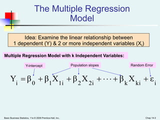
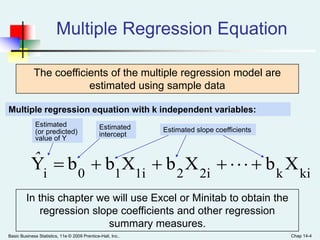
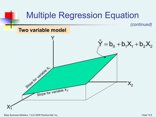
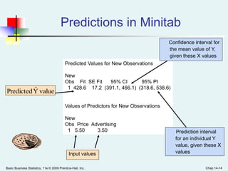
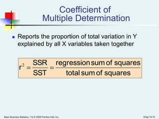
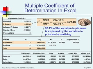
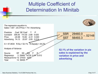
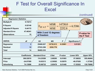
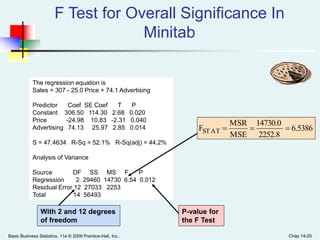
This document provides an overview of multiple regression analysis. It introduces the concept of using multiple independent variables (X1, X2, etc.) to predict a dependent variable (Y) through a regression equation. It presents examples using Excel and Minitab to estimate the regression coefficients and other measures from sample data. Key outputs include the regression equation, R-squared (proportion of variation in Y explained by the X's), adjusted R-squared (penalized for additional variables), and an F-test to determine if the overall regression model is statistically significant.

![Basic Business Statistics, 11e © 2009 Prentice-Hall, Inc.. Chap 14-57
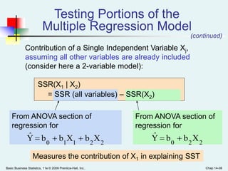
Simultaneous Contribution of
Independent Variables
Use partial F test for the simultaneous
contribution of multiple variables to the model
Let m variables be an additional set of variables
added simultaneously
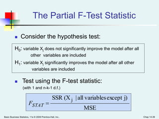
To test the hypothesis that the set of m variables
improves the model:
MSE(all)
m/)]variablesmofsetnewexcept(allSSR[SSR(all)
STATF
(where FSTAT has m and n-k-1 d.f.)](https://image.slidesharecdn.com/bbs11pptch14-200201163049/85/Bbs11-ppt-ch14-57-320.jpg)