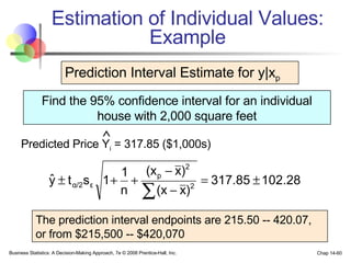
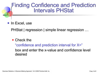
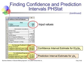
Downloaded 457 times

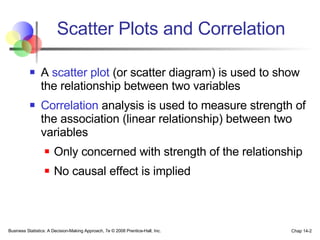
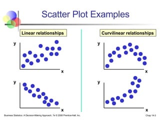
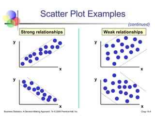
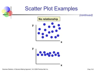
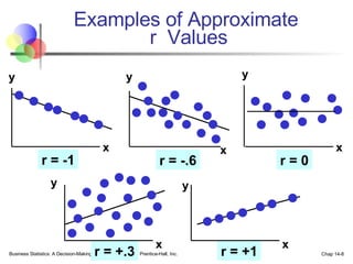
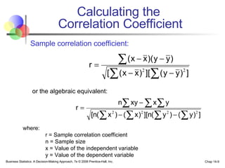
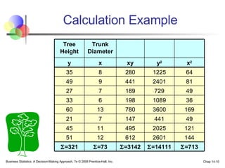
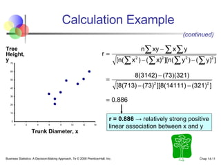
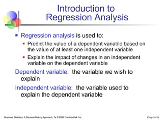
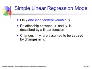
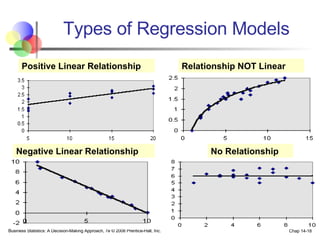
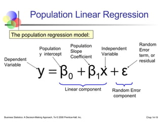
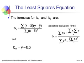
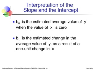
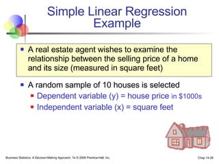
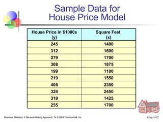
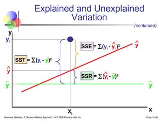
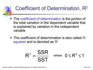
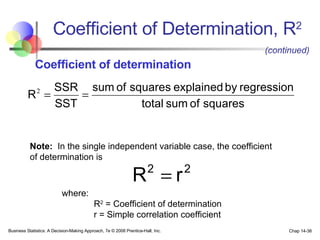
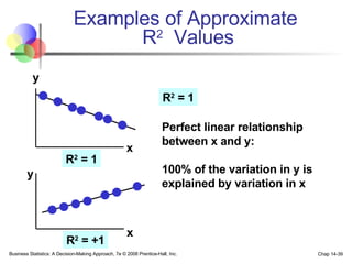
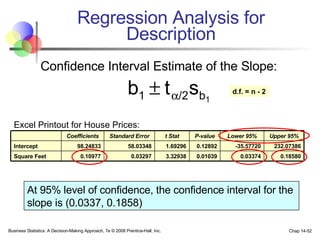
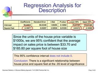
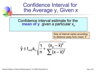
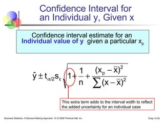

The document provides an introduction to linear regression and correlation analysis, detailing how scatter plots illustrate relationships between variables and how the correlation coefficient measures the strength of these relationships. It discusses regression analysis for predicting a dependent variable based on one or more independent variables and outlines the least squares method for estimating regression coefficients. The document also includes examples, calculations, and interpretations of statistical concepts such as the coefficient of determination (r²) and significance testing.