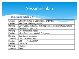
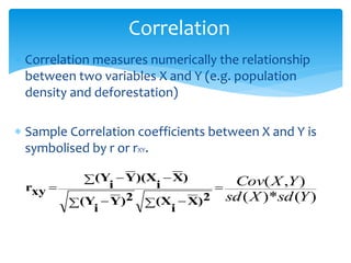
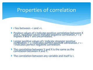
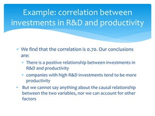
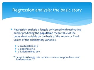
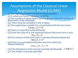
This document outlines the schedule and topics for an advanced econometrics and Stata training course taking place in Beijing from November 17-26, 2019. The course will cover topics including introduction to econometrics and Stata, single and multiple regression, hypothesis testing, time series models, panel data models, and frontier analysis. Sessions are planned each morning and evening, with exercises and practice sessions interspersed.

1. Advanced econometrics and Stata
L3-4 Data and Single regression
Dr. Chunxia Jiang
Business School, University of Aberdeen, UK
Beijing , 17-26 Nov 2019

2.  Topics and schedule
Sessions plan
Evening —
L1-2 Introduction to Econometrics and Stata
Evening —
L3-4 Data, single regression
Morning —
L5-6 Hypothesis testing, Multi-regression , Violation of assumptions
Afternoon Exercises and practice
Morning —
L7-8 Time series models
Evening —
L9-10 Panel data models & Endogeneity
Morning Exercises and practice
Afternoon L11-12 Frontier1 SFA
Evening L13-14： Frontier2 DEA
Evening L15-16 DID
Morning Revision
Afternoon Exam

3. Review: L1-2
 What is Econometrics?
 Methodology of econometrics
 Statement of theory or hypothesis
 Model definition
 Data
 Estimation
 Hypothesis testing
 Forecasting
 Policy simulation
 Introduction to STATA
 Portable, expandable, update available (SJ, Stata Technical Bulletin)
 Do file, data file

4.  Basic data analysis: Summary statistics
 One variable:
 Mean or average value
 Minimum and Maximum value
 Mode & Median
 Variance and standard deviation
 Two variables:
 Covariance
 Correlation
 Cross-plot (or scatter gram or scatter plot).
 Single regression
Preview: Data and simple regression

5. Basic Data Analysis
 Eyeballing the data helps establish presence of:
 trends versus mean reversion
 volatility clusters
 key observations
 outliers
 data errors?
 turning points
 regime changes

6. Outliers

7. Trends

8. More Trends

9. Basic Data Analysis
 All pieces of empirical work should begin with some basic
data analysis
 Eyeball the data
 Summarise the properties of the data series
 Examine the relationship between data series
 Most powerful analytic tools are your eyes and your
common sense
 Computers still suffer from “Garbage in - garbage out”

10. Basic Data Analysis (1)
 Summary statistics: particularly useful when cannot easily
look at the data, e.g., large panels or survey data
 Mean or average
 Minimum and Maximum value
Notation we normally use
for the mean of a
variable
N
Y
Y
N
i i
 
 1

11. Basic data analysis (2)
 Measure of dispersion
 Sample Variance:
 The variance shows how the individual values of a variable are
distributed around the mean of that variable. If all values are equal to
the mean, the variance is zero. If the values are widely spread around
the mean, variance will be large.
 Standard deviation
1
)
(
1
2



N
Y
Y
N
i
1
)
(
1
2


 
N
Y
Y
N
i
The standard deviation is particularly useful in a comparative sense. It is
always in the same units as the original sample data. It helps to know how a
set of data is distributed around its mean.
S2 =
S =

12. Example: Industry value added in
Millions of US $, 1992-2000
Mean SD Min Max
Agricult. 130,186 25,064 108,503 179,350
Mining 81,603 6,091 71,411 89,346
Food 102,184 8,241 90,699 119,794
Textile 52,704 3,950 46,388 57,558
Which sector has been more productive on average?
Which has been more volatile?
Why do you think this is the case?

13. Advanced descriptive statistics
 Mode: the most common value
 Median: the middle value in a set of data that has been ranked
from smallest to highest
 Percentile: divide the data set into 100 equal parts
 Quartile: divide the data range into four equal parts. The first
quartile separates the smallest 25% of the values from the other
75% that are larger. The second quartile is the median (50% of
the values are smaller than the median and 50% are higher)….
 Decile: divide the data up into ten groups.

14. Basic Data Analysis
 Since we are usually concerned with explaining one variable
using another, for example:
 “the use of the internet has made the market more
competitive”
 Relationships between variables are important
 cross-plots, multiple time-series plots
 correlations (covariances)

15. Example: XY-plot or scatter plot

16. Herfindahl index
 Herfindahl index (Herfindahl-Hirschman Index : HHI) :
the sum of the squares of the market shares of the
firms within the industry (sometimes limited to the
50 largest firms)
 It can range from 0 to 1 moving from a huge number
of small firms to a single monopolistic producer

17. Covariance
 Descriptive statistics for two variables
 Covariance: it measures how two variables move
together. It can be positive, negative or zero.
 Positive: the two variables move in the same direction
 Negative: the two variables move in opposite direction
 Zero: there is no relationship between the two variables.
 To calculate the sample co-variance:
 cov(X,Y) =
1
)
)(
(
1





n
Y
Y
X
X i
n
i
i

18. Covariance
 It tells us whether two variables are related.
 But it does not say anything about the strength of this
relationship.
 By itself not really very useful.

19. Correlation
 Correlation measures numerically the relationship
between two variables X and Y (e.g. population
density and deforestation)
 Sample Correlation coefficients between X and Y is
symbolised by r or rXY.
)
(
)*
(
)
,
(
Y
sd
X
sd
Y
X
Cov

 
 
 


2
)
X
i
(X
2
)
Y
i
(Y
)
X
i
)(X
Y
i
(Y
xy
r

20. Properties of correlation
 r lies between –1 and +1.
 Positive values of r indicate positive correlation between X
and Y, negative values indicate negative correlation, r = 0
implies X and Y are uncorrelated.
 Larger positive values of r indicate stronger positive
correlation. r = 1 indicates perfect positive correlation. r = -
1 indicates perfect negative correlation.
 The correlation between Y and X is the same as the
correlation between X and Y.
 The correlation between any variable and itself is 1.

21. Example: correlation between
investments in R&D and productivity
 We find that the correlation is 0.70. Our conclusions
are:
 There is a positive relationship between investments in
R&D and productivity
 companies with high R&D investments tend to be more
productivity
• But we cannot say anything about the causal relationship
between the two variables, nor we can account for other
factors

22. Regression analysis: the basic story
 Regression analysis is largely concerned with estimating
and/or predicting the population mean value of the
dependent variable on the basis of the known or fixed
values of the explanatory variables.
 y is a function of x
 y depends on x
 y is determined by x
“the spot exchange rate depends on relative price levels and
interest rates…”

23. Regression and Correlation
 If we say y and x are correlated, it means that
we are treating y and x in a symmetric way.
 In regression, we treat the dependent variable
(y) and the independent variable(s) (x’s) very
differently
◦ The y variable is assumed to be random or “stochastic” in
some way, i.e. to have a probability distribution.
◦ The x variables are assumed to have fixed (“non-
stochastic”) values in repeated samples.

24. Deterministic versus stochastic
relationships
(1) y = 10 + 5x
 y is known exactly if x is known
 x is known exactly if y is known
 which is dependent variable here?
(2) y = 10 + 5x + u
 The term ‘u’ is the error or disturbance term and it contains all
factors affecting y other than x.

25. Errors
 Where does the error come from?
 Randomness of (human) nature
 men and markets are not machines
 Omitted variables
 men and markets are more complex than the models we use
to describe them. Everything else is captured by the error
term
 Principle of parsimony: keep the regression model as simple as
possible.
 Measurement error in y and/or X
 Specification error: wrong functional form

26.  We may also write a do-file in the do-file editor and execute it. The
 Do-File Editor icon on the Toolbar brings up a window in which we may
 type those same three commands, as well as a few more:
 sysuse uslifeexp
 describe
 summarize
 notes
 // average life expectancy, 1900-1949
 summarize le if year < 1950
 // average life expectancy, 1950-1999
 summarize le if year >= 1950
 After typing those commands into the window, the rightmost icon, with
 tooltip Do, may be used to execute them.
Exercise

27.  Numbers are stored as byte, int, long, float, or double,
with the default being float. byte, int, and long are
said to be of integer type in that they can hold only
integers.
Data type

28.  label
 label dataset:
 label variable:
 webuse hbp4
 describe
 label list
 label define yesno 0 "no" 1 "yes“
 label dir
label

29. Relationships
 We are talking about statistical relationships:
y = α + βx + u
 The term ‘u’ is the error or disturbance term
 It contains all factors affecting y other than x
 Omitted variables
 Measurement errors
 Wrong functional form
29

30. Population and sample
 Population: the whole sample space representing a
phenomenon we are interested in.
 Sample: section of the sample space.
 In econometrics we can only use samples. Starting from a
sample our aim is to draw conclusions concerning the whole
population.
 In real research we do not observe the whole population
relative to a certain event but we can only observe a sample
of that population.
 To analyse how firms’ output is affected by R&D investments in
the UK. The population is the total number of UK firms. We
generally have information on a subgroup of these firms, e.g.,
those who employ over 50 employees.

31. Population and sample
 POPULATION REGRESSION FUNCTION (PRF):
 Our objective is to get estimates of the unknown parameters alpha and
beta, given N observations on Y and X.
 SAMPLE REGRESSION FUNCTION (SRF)
 Given that the SRF is only an approximation of the PRF, can we find a
method or procedure that makes this approximation as close as
possible?
 How can we construct the SRF so that is as close as possible to ?
31

ˆ 
i
i
i u
X
Y 

 
 i=1,2,…n
i
i
i u
X
Y ˆ
ˆ
ˆ 

 


32. ORDINARY LEAST SQUARES (OLS)
Ordinary least Squares (OLS)!
 The most frequently used method.
 To start with we use a very simple model, the
Two Variable Linear Regression Model.
 What does ‘linear’ mean?
 Linear model:
 Non linear model:
 By linear model we mean a model linear in the parameters.
32
2
1
2
1
)
|
( X
X
Y
E i 
 

i
i X
X
Y
E 2
2
1
)
|
( 
 


33. Estimator
 An estimator is a rule (or formula) that tells how to
estimate the population parameter from the information
provided by the sample at hand.
 A particular numerical value obtained by the estimator in
an application is known as an estimate.
 We could use other rules but OLS is the best estimator,
when some specific conditions are met.
33

34. Estimating the Regression Coefficients
 How do we determine  and  ?
 Choose  and  so that the distances from the data
points to the fitted lines are minimised (so that the line
fits the data as closely as possible)
 The most common method used to fit a line to
the data is known as OLS (ordinary least
squares).
34

35. Estimating the regression
coefficients
Y
35
X
Y = wages, X = years of education
22
Yours
17
Mine
80
40

36. Ordinary Least Squares
 OLS
1. Take each vertical distance between the data point and the
fitted line
2. Square it
3. Minimise the total sum of the squares (hence least squares).
 The principle of OLS is to minimize the total sum of
squared errors, i.e. Min ut
2. (t=1,2,...n). Because the
error term can be positive as well as negative and the
total sum of errors would be zero. This is why we choose
the squared errors rather than the error.
36

37. Derivation of the OLS coefficients
 Since
ˆ
ˆ
ˆ
u = y - y = y - α - βx
t t t t t
2
2 ˆ
Min Min (4)
ˆ
(y - α - βx )
u
1 1
t t
n n
t
t t

 
 
37

38. From the minimisation procedure we
derive the two following expressions:
ˆ
ˆ
α= y - βx
38
2
( )( )
ˆ
( )
t t
t
x x y y
x x

 



 Very important to
remember !
Very important to
remember !

39. Residuals and fitted values
 We can write yt as the sum of the fitted values (y hat)
and the fitted residuals (u hat).
 Given the values of and we can obtain the
fitted values for Yi according to the equation:
 We can also derive the fitted values of the residuals (u
hat):
39
̂ 
ˆ
i
i x
y 
 ˆ
ˆ
ˆ 

i
i
i y
y
u ˆ
ˆ 


40. Example: the CAPM – Capital Asset
Pricing Model
 How can we estimate this model using OLS?
40
t
t
t
t
xxx rf
rf
rm
r 


 )
(
, 

)
(
, t
t
t
t
xxx rf
rm
rf
r 


 

Excess return on portfolio Excess return on the market

41. The data
• We have the following data on the excess returns on a fund
manager’s portfolio (“fund XXX”) together with the excess
returns on a market index:
• We want to find whether there is a relationship between Y and
X given the data that we have. The first stage would be to derive
a scatter plot of the two variables.
41
Year, t Excess return
= rXXX,t – rft
Excess return on market index
= rmt - rft
1 17.8 13.7
2 39.0 23.2
3 12.8 6.9
4 24.2 16.8
5 17.2 12.3

42. Graph (Scatter Diagram)
0
5
10
15
20
25
30
35
40
45
0 5 10 15 20 25
Excess
return
on
fund
XXX
Excess return on market portfolio
42
The main purpose of regression analysis is to find the line that best fits this
scatter of points
This point refers
To year 2

43. What do we use and for?
• In the CAPM example used above, optimizing would lead to
the estimates
• = -1.74 and = 1.64.
• We would write the fitted line as:
 If an analyst tells you that she expects the market to yield a
return 20% higher than the risk-free rate next year, what
would you expect the return on fund XXX to be?
• Solution: We can say that the expected value of
y = “-1.74 + 1.64 * value of x”, so plug x = 20 into the equation
to get the expected value for y:
43
$

$
 $

t
t x
y 64
.
1
74
.
1
ˆ 


$

06
.
31
20
64
.
1
74
.
1
ˆ 




i
y

44. Deriving fitted values
 Let’s go back to the estimated CAPM model:
Rxxx Rm
Year Yt Xt Yt hat Ut hat
2000 17.80 13.70 20.76 -2.96
2001 39.00 23.20 36.35 2.65
2002 12.80 6.90 9.59 3.21
2003 24.20 16.80 25.84 -1.64
2004 17.20 12.30 18.46 -1.26
44
t
t x
y 64
.
1
74
.
1
ˆ 



45. Actual and fitted values
0.00
5.00
10.00
15.00
20.00
25.00
30.00
35.00
40.00
45.00
2000 2001 2002 2003 2004
Y
Yhat
Actual and fitted values in the CAPM
model
45
Year

46. How do we tell that OLS is a good
estimator of the PRF?
 We need to make some assumptions about the explanatory variable
(x) and the error term (u) otherwise we will not be able to tell how
good a SRF is as an estimate of the PRF.
 If our objective is to estimate the parameters only then the
method of OLS – what we have done so far, will be enough.
 However we want to draw inferences about their true values.
 How close our estimated beta 1 and beta2 are to the their
counterparts in the population.
 We need to make certain assumptions about Xi and the error term.
These assumptions are critical to the valid interpretation of the
regression estimates.
46

47. Assumptions of the Classical Linear
Regression Model (CLRM)
 (1) The regression model is linear in the parameters.
 (2) X values are fixed in repeated sampling.
 (3) The number of observations must be greater than the number of
parameters to be estimated.
 (4) There must be variability in the X values.
 (5) The explanatory variable X is uncorrelated with the error term:
 (6) There is no perfect multicollinearity.
 (7) Given the value of X, the expected value of the error term is zero
 (8) The variance of the error term is constant (homoscedasticity).
 (9) There is no correlation between two error terms (no
autocorrelation).
 (10) The disturbance term must be normally distributed
 (11) The model is correctly specified.
47
0
)
|
( 
X
u
E
0
)
,
( 
i
i X
u
Cov
2
)
var( 

i
i X
u
0
)
,
,
cov( 
j
i
j
i X
X
u
u
)
σ
N(0,
u 2
t 

48. Another way of looking at our regression
 Given that:
 By rearranging, we can write the following:
 This shows that OLS decomposes each
observation (yi) into two parts:
 A fitted value (the explained component)
 A residual (the unexplained component)
48
i
i
i y
y
u ˆ
ˆ 

i
i
i u
y
y ˆ
ˆ 


49. Three useful sums:
 Total Sum of Squares (SST):
 Explained Sum of Squares (SSE):
 Residuals Sum of Squares (SSR):
49




n
i
i y
y
SST
1
2
)
(




n
i
i y
y
SSE
1
2
)
ˆ
(



n
i
i
u
SSR
1
2
ˆ

50. Goodness-of-Fit
 It is easy to prove that: SST = SSE + SSR
 R-squared or coefficient of determination:
 This tells us the fraction of the sample variation in y
that is explained by x.
 R-square is always between 0 and 1.
 We usually multiply it by 100 so we can talk in terms
of percentage: R2 is the percentage of the sample
variation in y that is explained by x.
50
SST
SSE
R /
2


51. Characteristics of R-square
 R-square = 1 we have a perfect fit. Usually a
suspicious result!!!
 R-square = 0 our model cannot explain any of the
variation in the data. None of the variation in yi is
captured by y hat.
 We can use it as an indication of the goodness of
our model but we have to be careful because:
 The model could still be valid under certain
circumstances. For example: studies based on cross-
sectional data usually produce low R-square values.
51

52. From univariate to multivariate
regression analysis
 With multivariate regression analysis we can control for
several factors affecting our dependent variable.
 We have to pay particular attention to:
 (1) the independent variables (Xs);
 (2) the relationship among these variables (Xs);
 (3) the relationship between these variables (Xs) and the
dependent variable (Y).
52

53. Interpretation of the slope coefficients or partial
regression coefficients
 Each estimated coefficient measure the impact of the
respective variable on the dependent variable, holding
everything else fixed (the other variables are held fixed).
 More technically, if we have:
 Beta 2 measures the change in Y given a one-unit increase in X2
 Beta 3 measures the change in Y given a one-unit increase in X3
 They are called the partial regression coefficients
 We control for the impact of other variables in estimating,
for example, the effect of X2 on Y.
 We can still compute the change in Y when two or more
independent variables change.
)
1
(
e
X
β
X
β
β
Y t
3t
3
2t
2
1
t 



53

54. R2
 R-square gives the proportion of the total variation in Yi
explained by the independent variables jointly.
 Adjusted R-square: it controls for the number of
explanatory variables included in the model (adjusted
for df)
 The more variables in the model the larger the R-
square, adjusted R-square increases less than the
unadjusted one





 2
2
2
)
(
ˆ
1
/
Y
Y
u
SST
SSE
R
i
i







)
1
/(
)
(
)
/(
ˆ
1 2
2
2
n
Y
Y
k
n
u
R
i
i
54

55. Statistical inference
 Statistical inference is concerned with drawing
conclusions about the nature of some
population on the basis of a random sample that
has been drawn from that population.
 Estimation is the first step of statistical inference
 Having obtained an estimate of a parameter we
need to find out how good that estimate is.
55

56. Statistical inference and R2
 The coefficient of determination gives us a first indication of
how good our estimates are.
 It tells us the proportion of the variation in Y which is
explained by variations in X.
 If R2 = 0.80 this means that the regression line gives a good
fit to the observed data since it explains 80% of the variation
of the Y values around their mean.
 The remaining 20% is attributed to the factors included in the
disturbance term.
56

57. Seminar question:
Q1: Students’ coursework results
 Results for the first econometric coursework. We have a
sample of 12 students.
Student n. Coursework 1
1 60 Maximum
2 24 Minimum
3 68 Average (mean)
4 60 Mode
5 70 Median
6 65
7 76
8 52
9 70
10 40
11 60
12 68
13 55

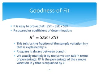
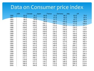
58. Q2: Inflation rate
 This is an excel based exercise
 Using table below, compute the inflation rate for 7
industrialized countries.
 Subtract from the current year’s CPI the CPI of the
previous year, divide the difference by the previous
year’s CPI, and multiply the result by 100.
 For example, the inflation rate for Canada for 1981 is
[(85.6-76.1)/76.1]*100=12.48%

59. Data on Consumer price index
USA Canada Japan France Germany Italy UK
1980 82.4 76.1 90.9 72.3 86.7 63.2 78.5
1981 90.9 85.6 95.3 81.9 92.2 75.4 87.9
1982 96.5 94.9 98.1 91.7 97.1 87.7 95.4
1983 99.6 100.4 99.8 100.4 100.3 100.8 99.8
1984 103.9 104.7 102.1 108.1 102.7 111.5 104.8
1985 107.6 109.0 104.2 114.4 104.8 121.1 111.1
1986 109.6 113.5 104.9 117.3 104.7 128.5 114.9
1987 113.6 118.4 104.9 121.1 104.9 134.4 119.7
1988 118.3 123.2 105.6 124.4 106.3 141.1 125.6
1989 124.0 129.3 108.0 128.7 109.2 150.4 135.3
1990 130.7 135.5 111.4 133.0 112.2 159.6 148.2
1991 136.2 143.1 115.0 137.2 116.3 169.8 156.9
1992 140.3 145.3 117.0 140.5 122.1 178.8 162.7
1993 144.5 147.9 118.5 143.5 127.6 186.4 165.3
1994 148.2 148.2 119.3 145.8 131.1 193.7 169.4
1995 152.4 151.4 119.2 148.4 133.5 204.1 175.1
1996 156.9 153.8 119.3 151.4 135.5 212.0 179.4
1997 160.5 156.3 121.5 153.2 137.8 215.7 185.0
1998 163.0 157.8 122.2 154.2 139.1 222.5 191.4
1999 166.6 160.5 121.8 155.0 140.0 226.2 194.3
2000 172.2 164.9 121.0 157.6 142.0 231.9 200.1
2001 177.1 169.1 120.1 160.2 144.8 238.3 203.6
2002 179.9 172.9 119.0 163.3 146.7 244.3 207.0
2003 184.0 177.7 118.7 166.7 148.3 250.8 213.0
2004 188.9 181.0 118.7 170.3 150.8 256.3 219.4
2005 195.3 184.9 118.3 173.2 153.7 261.3 225.6