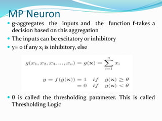
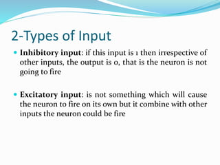
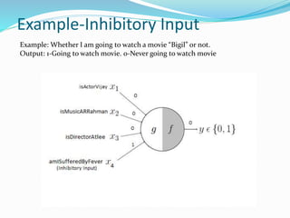
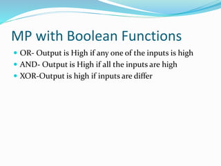
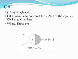
The document discusses the history and concepts of artificial intelligence and machine learning. It describes early models like the McCulloch-Pitts neuron and perceptron, and how they evolved with the introduction of backpropagation and multi-layer perceptrons using sigmoid activation functions. Key algorithms discussed include naive Bayes, k-means clustering, and decision trees. Deep learning concepts like convolutional neural networks are also covered at a high level.

1. S.B.S.Younus,
M.Phil-Computer Science,
Sadakathullah Appa College.

2. Introduction
 Artificial Intelligence is a technology that make
computers to act like human
 Artificial Intelligence is an umbrella term. In which
there are many subfields. They are,
 Machine Learning
 Deep Learning
 Big Data
 Cloud Computing

3. Machine Learning
 Machine Learning is a technique that makes computer
to take decisions or to solve problems without being
explicitly programmed
 Machine learns from experience that is it learns from
data

4. ML Algorithms
 Naïve Bayes Classifier Algorithm
 K Means Clustering Algorithm
 Support Vector Machine Algorithm
 Apriori Algorithm
 Linear Regression
 Logistic Regression
 Artificial Neural Networks
 Random Forests
 Decision Trees
 Nearest Neighbours

5. Deep Learning
 Learn something in –depth
 DL Uses Artificial Neural Network (ANN) to make
decision or to solve problem
 ANN-based on Biological Neural Network (BNN)

6. BNN & ANN Abstract

7. BNN
 Dendrite: Receives signals from other neurons
 Soma: Processes the information
 Axon: Transmits the output of this neuron
 Synapse: Point of connection to other neurons

8. ANN
 Neuron: Basic computational unit of ANN
 Input Layer: Receives input from the dataset. Number
of inputs refers the number of features
 Hidden layer: The hidden layers greatly contributes
to the performance of the model. A network can have a
single hidden layer or many hidden layers which are
connected together.
 Output Layer: Outcome of the model

9. Types
 The type of hidden layer distinguishes the different
types of Neural Networks
 ANN
 CNN
 RNN
 The number of hidden layers is termed as the depth of
the neural network

10. Evolution
 McCulloch Pitts Neuron
 Perceptron
 Sigmoid Neurons

11. MP Neuron
 McCulloch-Pitts Neuron — Mankind’s First
Mathematical Model Of a Biological Neuron
 McCulloch (neuroscientist) and Pitts (logician)
proposed a highly simplified computational model
of the neuron (1943)
 Input and Output is binary

12. MP Neuron

13. MP Neuron
 g-aggregates the inputs and the function f-takes a
decision based on this aggregation
 The inputs can be excitatory or inhibitory
 y= 0 if any xi is inhibitory, else
 θ is called the thresholding parameter. This is called
Thresholding Logic

14. 2-Types of Input
 Inhibitory input: if this input is 1 then irrespective of
other inputs, the output is 0, that is the neuron is not
going to fire
 Excitatory input: is not something which will cause
the neuron to fire on its own but it combine with other
inputs the neuron could be fire

15. Example-Inhibitory Input
Example: Whether I am going to watch a movie “Bigil” or not.
Output: 1-Going to watch movie. 0-Never going to watch movie

16. MP with Boolean Functions
 OR- Output is High if any one of the inputs is high
 AND- Output is High if all the inputs are high
 XOR-Output is high if inputs are differ

17. OR
 g(X)=g(x1, x2)=x1+x2
 OR function neuron would fire if ANY of the inputs is
ON i.e., g(X) ≥ 1 here.
 Where, Theta-ϴ=1

18. OR-Table

19. OR-Geometric Interpretation

20. AND
 g(X)=g(x1, x2)=x1+x2
 OR function neuron would fire if ANY of the inputs is
ON i.e., g(X) ≥ 2 here.
 Where, Theta-ϴ=2

21. AND- Truth Table

22. AND-Geometric Interpretation

23. Linear Separability
 A single McCulloch Pitts Neuron can be used to
represent boolean functions which are linearly
separable.
 Linear separability (for boolean functions) :
There exists a line (plane) such that all inputs
which produce a 1 lie on one side of the line
(plane) and all inputs which produce a 0 lie on other
side of the line (plane)
 MP Neuron is not applicable for XOR. Because, XOR is
non linearly separable function

24. XOR-Linearly Non-Separable

25. Limitations of MP Neuron
 What about non-boolean (say, real) inputs?
 Are all inputs equal? What if we want to assign more
importance to some inputs?
 What about functions which are not linearly
separable? Say XOR function.

26. Perceptron
 Frank Rosenblatt, an American psychologist, proposed
the classical perceptron model(1958)
 A more general computational model than
McCulloch–Pitts neurons
 Main differences: Introduction of numerical
weights for inputs and a mechanism for learning
these weights
 Input-Real Value
 Output- Binary (0,1)

27. Perceptron
 It takes an input, aggregates it (weighted sum) and
returns 1 only if the aggregated sum is more than some
threshold else returns 0
 Perceptron is usually used to classify the data into two
parts. Therefore, it is also known as a Linear Binary
Classifier.

28. Perceptron

29. Bias
 In the above diagram, x0 is bias input.
 Bias is an additional parameter in the Neural Network
which is used to adjust the output along with the
weighted sum of the inputs to the neuron.
 Therefore Bias is a constant which helps the model in a
way that it can fit best for the given data.
 bias helps in controlling the value at which activation
function will trigger

30. OR with Perceptron

31. Learning Algorithm

32. MLP
 Multi-layer Perceptron model (MLP) is an artificial
neural network with three or more hidden layers.
 It is a feed-forward neural network that uses back
propagation technique for training the network.
 Multi-layer perceptron model is sometimes referred to
as the deep neural network because it has many
hidden layers.

33. MLP
 It is a deep learning method used for supervised
learning and its capable of modeling complex
problems.
 Multi-layer perceptron is capable of handling both
linearly and non-linearly separable tasks.

34. MLP

35. MLP
 There are 2 stages in learning process
 Feedforward
 Backpropagation

36. Feedforward
 The input layer receives the features from the data set
each node representing a feature
 bias is added to the sum of input and weight
 The information from the input layer is sent to each
neuron in the hidden layer for further processing

37.  The neurons in the hidden layer accepts the
information from input layer together with their
weights and biases.
 The neuron has an activation function which regulates
the processing of information in the neuron
 The activation function ensures that the information is
within the required range such as 0 to 1 or -1 to 1

38.  The output from one layer is the input in the next
layer.
 When the information moves from one layer to the
next layer it is multiplied by the weights and bias
added.
 The final hidden layer is the output layer and is
responsible for predicting the results of the model

39. Backpropagation
 We can improve the accuracy of the prediction
by adjusting weights and biases in a backward
direction.
 The objective of back propagation is to reduce the
error
 Error(loss function)=Expected Output-Actual
Output
 There are many types of loss functions such as
 Root Mean Squared Error (RMES)
 Cross Entropy (CE)

40.  The error is reduced through what is called the
gradient descent process which uses the
derivatives to find the gradient/slope of the error
function
 The objective of gradient descent is to move the error
to the zero level

41. Sigmoid Neurons
 Why Sigmoid Neuron?
 MP-Neuron
 Input and Output= Binary
 Perceptron
 Input=Real value, Output=Binary
 Can’t handle linearly non-separable problems
 MLP(Network of Perceptron)
 Input=Real value, Output=Binary
 Can handle linearly non-separable problems

42. Sigmoid Neuron
 Both input and Output are real values
 Output of sigmoid neuron is a real value between 0
and 1, which is smoother than binary input
 There are many functions with the characteristic of an
“S” shaped curve known as sigmoid functions
 The most commonly used function is the logistic
function

49. Learning Algorithm
 The objective of the learning algorithm is to determine
the best possible values for the parameters (w and b),
such that the overall loss (squared error loss) of the
model is minimized as much as possible.

50. Algorithm

51. Gradient Descent
 Gradient Descent is an optimization algorithm used for
minimizing the cost function in various machine learning
algorithms. It is basically used for updating the parameters
of the learning model
 Gradient Descent can be described as an iterative method
which is used to find the values of the parameters of a
function that minimizes the cost function as much as
possible. The parameters are initially defined a particular
value and from that, Gradient Descent is run in an iterative
fashion to find the optimal values of the parameters, using
calculus, to find the minimum possible value of the given
cost function.

52. Types
 Batch Gradient Descent
 The batch is taken to be the whole dataset. batch” which
denotes the total number of samples from a dataset.
The problem arises when our datasets get really huge.
 Stochastic Gradient Descent
 The word ‘stochastic‘ means a system or a process that is
linked with a random probability. Hence, in Stochastic
Gradient Descent, a few samples are selected
randomly instead of the whole data set for each
iteration

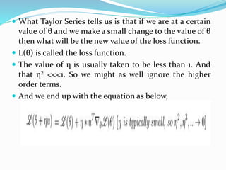
53. Geometric Interpretation
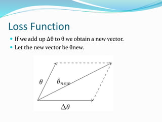
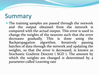
 Our main objective is to navigate through the error
surface inorder to reach a point where the error is less
or close to zero.
 Let us assume θ = [w,b] where w & b are the weights
and the biases respectively. θ is an arbitrary point on
the error surface.To start with w & b are randomly
initialized and this is our starting point.
 θ is a vector of parameters w and b such that θ ∈ R².

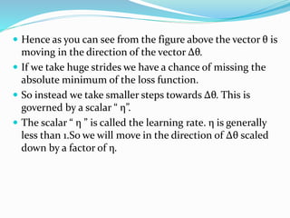
54.  Let us assume Δθ = [Δw , Δb] where Δw & Δb are the
changes that we make to the weights and biases such
that we move in the direction of reduced loss and land
up at places where the error is less. Δθ is a vector in the
direction of reduced loss.
 Δθ is a vector of parameters Δw and Δb such that Δθ ∈
R².
 Now we need to move from θ to θ+Δθ such that we
move towards the direction of minimum loss

55. Loss Function
 If we add up Δθ to θ we obtain a new vector.
 Let the new vector be θnew.

56.  Hence as you can see from the figure above the vector θ is
moving in the direction of the vector Δθ.
 If we take huge strides we have a chance of missing the
absolute minimum of the loss function.
 So instead we take smaller steps towards Δθ. This is
governed by a scalar “ η”.
 The scalar “ η ” is called the learning rate. η is generally
less than 1.So we will move in the direction of Δθ scaled
down by a factor of η.

57.  Hence, θnew = θ + η.Δθ where Δθ is the direction of
reduced loss.
 So we start from a random value of θ. And then we move
in the direction of Δθ which ensures that our loss
decreases. And we need to do this in a cyclic manner to
reach the global minimum.

58.  But what is Δθ ? And what is the right value for Δθ?
 So the answer for the question above comes from Taylor
Series.
 For simpicity, lets assume Δθ =u . And here we go.

59.  What Taylor Series tells us is that if we are at a certain
value of θ and we make a small change to the value of θ
then what will be the new value of the loss function.
 L(θ) is called the loss function.
 The value of η is usually taken to be less than 1. And
that η² <<<1. So we might as well ignore the higher
order terms.
 And we end up with the equation as below,

60.  So we have some value of θ and we want to move away
from that direction such that the new loss L(θ+ηu) is
less than the old loss L(θ).
 So a desired value for “ u ” is obtained when the
following condition holds.

61.  This implies,
This condition should hold for the vector u that we
are trying to choose so that we can be sure that we
have chosen a good value for “ u ”. A good value of “ u
” can be obtained if the loss of the new step is less
than the loss of the previous step

62. Feedforward Neural Network
 As the name suggests, the input data is fed in the
forward direction through the network. Each hidden
layer accepts the input data, processes it as per the
activation function and passes to the successive layer.
 At each neuron in a hidden or output layer, the
processing happens in two steps:
 Preactivation
 Activation

63.  Preactivation
 it is a weighted sum of inputs
 Based on this aggregated sum and activation function
the neuron makes a decision whether to pass this
information further or not.
 Activation
 It ensures that the information is within the required
range such as 0 to 1 or -1 to 1
 Popular Activation Functions
 Sigmoid
 Hyperbolic
 tangent(tanh)
 ReLU
 Softmax

64. Sigmoid

65. Tanh

66. ReLU

67. Summary
 The training samples are passed through the network
and the output obtained from the network is
compared with the actual output. This error is used to
change the weights of the neurons such that the error
decreases gradually. This is done using the
Backpropagation algorithm, Iteratively passing
batches of data through the network and updating the
weights, so that the error is decreased, is known as
Stochastic Gradient Descent ( SGD ). The amount by
which the weights are changed is determined by a
parameter called Learning rate