Downloaded 48 times

![Adaptive Resonance Theory
Grossberg, S. (1976a). Adaptive pattern classification and univer-
sal recoding I: Feedback, expectation, olfaction, illusions. Biological
Cybernetics, 23: 187–202.
a “neural network that self–organize[s] stable pat-
tern recognition codes in real time, in response to
arbitrary sequences of input patterns”.
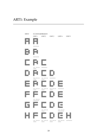
ART1 (1976). Localist representation, binary patterns.
ART2 (1987). Localist representation, analog patterns.
ART3 (1990). Distributed representation, analog pat-
terns.
Desirable properties:
plastic + stable
biological mechanisms
analytical math foundation
16](https://image.slidesharecdn.com/som-090922025047-phpapp02/85/redes-neuronales-tipo-Som-16-320.jpg)

This document discusses self-organizing neural networks, including Kohonen networks and Adaptive Resonance Theory (ART). It provides details on Kohonen networks such as their basic structure, learning algorithm using neighborhoods, and biological origins. ART is introduced as a way to address the stability-plasticity dilemma in neural networks. The key aspects of ART1 are summarized, including its orienting and attentional subsystems, short and long term memory representations, and learning algorithm using a vigilance test. Examples of a Kohonen network and ART1 network are also included to illustrate their operation.


![Competitive Learning [Deep Learning And Nueral Networks].pptx](https://cdn.slidesharecdn.com/ss_thumbnails/competitivelearning-240211053020-bc9a8437-thumbnail.jpg?width=640&height=640&fit=bounds)


