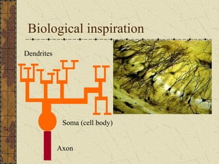
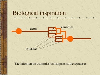
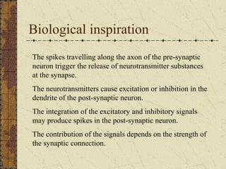
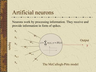
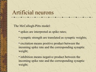
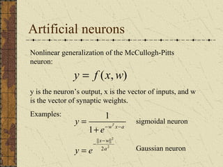
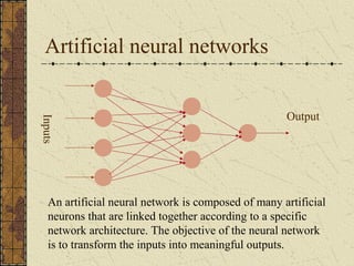
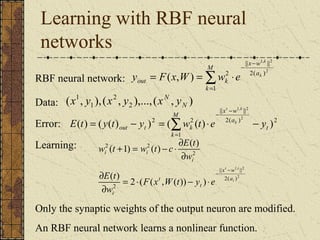
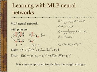
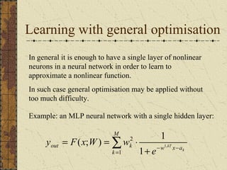
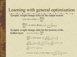
This document discusses artificial neural networks and their learning processes. It provides an overview of biological inspiration for neural networks from the nervous system. It then describes artificial neurons and how they are modeled, including the McCulloch-Pitts model. Neural networks are composed of interconnected artificial neurons. Learning in neural networks and biological systems involves changing synaptic strengths. The document outlines learning rules and processes for artificial neural networks, including minimizing an error function through optimization techniques like backpropagation.

1. Artificial Neural Networks
- Introduction -
Peter Andras
peter.andras@ncl.ac.uk

2. Overview
1. Biological inspiration
2. Artificial neurons and neural networks
3. Learning processes
4. Learning with artificial neural networks

3. Biological inspiration
Animals are able to react adaptively to changes in their
external and internal environment, and they use their nervous
system to perform these behaviours.
An appropriate model/simulation of the nervous system
should be able to produce similar responses and behaviours in
artificial systems.
The nervous system is build by relatively simple units, the
neurons, so copying their behavior and functionality should be
the solution.

4. Biological inspiration
Dendrites
Soma (cell body)
Axon

5. Biological inspiration
axon dendrites
synapses
The information transmission happens at the synapses.

6. Biological inspiration
The spikes travelling along the axon of the pre-synaptic
neuron trigger the release of neurotransmitter substances
at the synapse.
The neurotransmitters cause excitation or inhibition in the
dendrite of the post-synaptic neuron.
The integration of the excitatory and inhibitory signals
may produce spikes in the post-synaptic neuron.
The contribution of the signals depends on the strength of
the synaptic connection.

7. Artificial neurons
Neurons work by processing information. They receive and
provide information in form of spikes.
n
i i = =å=
z w x y H z
The McCullogh-Pitts model
Inputs
w1
w Output 2
w3
wn
wn-1
. . .
x1
x2
x3
…
xn-1
xn
y
; ( )
1
i

8. Artificial neurons
The McCullogh-Pitts model:
• spikes are interpreted as spike rates;
• synaptic strength are translated as synaptic weights;
• excitation means positive product between the
incoming spike rate and the corresponding synaptic
weight;
• inhibition means negative product between the
incoming spike rate and the corresponding synaptic
weight;

9. Artificial neurons
Nonlinear generalization of the McCullogh-Pitts
neuron:
y = f (x,w)
y is the neuron’s output, x is the vector of inputs, and w
is the vector of synaptic weights.
Examples:
y T
= sigmoidal neuron
- -
x w
|| ||
2
2
2
1
1
a
w x a
y e
e
- -
=
+
Gaussian neuron

10. Artificial neural networks
Inputs
Output
An artificial neural network is composed of many artificial
neurons that are linked together according to a specific
network architecture. The objective of the neural network
is to transform the inputs into meaningful outputs.

11. Artificial neural networks
Tasks to be solved by artificial neural networks:
• controlling the movements of a robot based on self-perception
and other information (e.g., visual
information);
• deciding the category of potential food items (e.g.,
edible or non-edible) in an artificial world;
• recognizing a visual object (e.g., a familiar face);
• predicting where a moving object goes, when a robot
wants to catch it.

12. Learning in biological systems
Learning = learning by adaptation
The young animal learns that the green fruits are sour,
while the yellowish/reddish ones are sweet. The learning
happens by adapting the fruit picking behavior.
At the neural level the learning happens by changing of the
synaptic strengths, eliminating some synapses, and
building new ones.

13. Learning as optimisation
The objective of adapting the responses on the basis of the
information received from the environment is to achieve a
better state. E.g., the animal likes to eat many energy rich,
juicy fruits that make its stomach full, and makes it feel
happy.
In other words, the objective of learning in biological
organisms is to optimise the amount of available resources,
happiness, or in general to achieve a closer to optimal state.

14. Learning in biological neural
networks
The learning rules of Hebb:
• synchronous activation increases the synaptic strength;
• asynchronous activation decreases the synaptic
strength.
These rules fit with energy minimization principles.
Maintaining synaptic strength needs energy, it should be
maintained at those places where it is needed, and it
shouldn’t be maintained at places where it’s not needed.

15. Learning principle for
artificial neural networks
ENERGY MINIMIZATION
We need an appropriate definition of energy for artificial
neural networks, and having that we can use
mathematical optimisation techniques to find how to
change the weights of the synaptic connections between
neurons.
ENERGY = measure of task performance error

16. Neural network mathematics
Inputs
Output
y f x w
( , )
=
y f x w
( , )
=
y f x w
( , )
1
( , )
4 4
1
4
1
3 3
1
3
1
2 2
1
2
1
1 1
1
1
=
y =
f x w
2
1
2 1
1
y f y w
( , )
ö
æ
=
2
3
y
y ( , 3 )
2
2
=
2 1
2
y f y w
( , )
2
3
=
2 1
3
y f y w
( , )
=
ö
÷ ÷ ÷ ÷ ÷
ø
æ
=
ç ç ç ç ç
è
1
1
1
2
1
3
1
4
1
y
y
y
y
y f y2 w Out =
1
÷ ÷ ÷ ÷
ø
ç ç ç ç
è
2
3
2
3
2
y
y
y

17. Neural network mathematics
Neural network: input / output transformation
yout = F(x,W)
W is the matrix of all weight vectors.

18. MLP neural networks
MLP = multi-layer perceptron
Perceptron:
y wT x
out = x yout
MLP neural network:
x yout
k
k
T
3 2
k w x a
1 1
e
y
- -
y y y y
( , , )
=
k w y a
e
y
y y y
2
=
out k k
1
2
2
3 2
2
1
1
2
2
1
3
1
2
1
1
1
( , )
, 1,2
1
1
, 1,2,3
1
1
2 1 2
y w y w y
k
T
T
k
kT
k
kT
= =
=
+
=
=
+
=
å=
- -

19. RBF neural networks
RBF = radial basis function
r x = r x -
c
( ) (|| ||)
x w
- -
=
|| ||
2
2
2
( )
a
f x e
Example: Gaussian RBF
x
yout
4
å=
x w
- -
1, 2
2 2
= ×
1
|| ||
2( )
k
a
out k
k
k
y w e

20. Neural network tasks
• control
• classification
• prediction
• approximation
These can be reformulated
in general as
FUNCTION
APPROXIMATION
tasks.
Approximation: given a set of values of a function g(x)
build a neural network that approximates the g(x) values
for any input x.

21. Neural network approximation
Task specification:
Data: set of value pairs: (xt, yt), yt=g(xt) + zt; zt is random
measurement noise.
Objective: find a neural network that represents the input /
output transformation (a function) F(x,W) such that
F(x,W) approximates g(x) for every x

22. Learning to approximate
Error measure:
1 N
( ( ; ) )2
å=
= -
t
F xt W yt
N
E
1
Rule for changing the synaptic weights:
w c E
D = - × ¶
j
i
w w w
j
i
j
i
j new
i
j
i
W
w
¶
= + D
,
( )
c is the learning parameter (usually a constant)

23. Learning with a perceptron
Perceptron: y wT x
out =
2
Data: ( , 1
),( , 2 ),...,( , )
1
N
x y x y xN y
T t
Error: E ( t ) = ( y ( t ) out - yt )2 = ( w ( t ) x - y
2 t
)Learning:
w t c w t x y
w t + = w t - c × ¶
E t
w ( t + 1) = w ( t ) - c × ( w ( t ) x - y )
×
x
t
j
m
j
j
T
t
t i
T t
i i
¶ -
i
t
T t
i
i
i i
w t x w t x
w
w
= ×
¶
= - ×
¶
å=
1
2
( ) ( )
( ( ) )
( 1) ( ) ( ) ( )
A perceptron is able to learn a linear function.

24. Learning with RBF neural
networks
M
1, 2
2 2
y = F ( x , W )
= w ×
e
RBF neural network:
Data: ( 1
, 1
),( 2
, 2 ),...,( , )
out k
N
x y x y xN y
x w
- -
t k
|| ||
1, 2
x w
å=
1
- -
|| ||
k
a
2( )
- × = - = å=
k
k
( ) ( ( ) )2 ( 2 ( ) ) 2
Error: 2
1
2( )
t
M
k
a
E t y t out yt wk t e y k
Learning:
t i
a
1, 2
x w
|| ||
2
2( )
w t + = w t - c × ¶
E t
( 1) ( ) ( )
E t
2
2
2 2
( ) 2 ( ( , ( )) )
i
t
t
i
i
i i
F x W t y e
w
w
- -
= × - ×
¶
¶
¶
Only the synaptic weights of the output neuron are modified.
An RBF neural network learns a nonlinear function.

25. Learning with MLP neural
networks
MLP neural network:
with p layers
2
e
y
kT
y y y
e
y
kT
y y y
Data: ( , 1
),( , 2 ),...,( , )
1
N
x y x y xN y
t
k w x a
1 1
- -
k
( ,..., )
k w y a
2 1 2
=
=
Error: E ( t ) = ( y ( t ) 2 out - yt )= ( F ( x ; W ) - y
)2
t k M
k M
1
2 2
1
2
2
2
1 1
1
1
1
1
( ; )
...
( ,..., )
, 1,...,
1
1
, 1,...,
1
1
2
1
-
- -
= =
=
+
=
=
+
=
pT p
out
k
T
M
T
M
y F x W w y
It is very complicated to calculate the weight changes.
x
yout
1 2 … p-1 p

26. Learning with backpropagation
Solution of the complicated learning:
• calculate first the changes for the synaptic weights
of the output neuron;
• calculate the changes backward starting from layer
p-1, and propagate backward the local error terms.
The method is still relatively complicated but it
is much simpler than the original optimisation
problem.

27. Learning with general optimisation
In general it is enough to have a single layer of nonlinear
neurons in a neural network in order to learn to
approximate a nonlinear function.
In such case general optimisation may be applied without
too much difficulty.
Example: an MLP neural network with a single hidden layer:
M
( ; ) 1
å=
out k w x a
+ - -
= = ×
k
k
kT e
y F x W w
1
2
1, 1

28. Learning with general optimisation
Synaptic weight change rules for the output neuron:
i
( ) 2 ( ( , ( )) ) 1
t w iT xt a
w t + = w t - c × ¶
E t
t
E t
i
i
i i
e
F x W t y
w
w
+ - -
= × - ×
¶
¶
¶
1, 1
( 1) ( ) ( )
2
2
2 2
Synaptic weight change rules for the neurons of the
hidden layer:
w 1, ( t + 1) = w 1,
( t ) - c × ¶
E ( t
)
1,
E t
= × - × ¶
( ) 2 ( ( , ( )) ) 1
1
1, 1,
w x a
ö
æ
- -
( ) ( )
1
ö
1 1
æ
( )
w x a
e
- - = -
× ¶
¶
¶
w t w t c F x W t y e
- -
( ) ( )
1
1,
1,
( 1) ( ) 2 ( ( , ( )) )
2
1, 1,
1,
1, 2 1,
1,
1,
1,
1,
1,
1,
t
j
w x a
t
i t
j
i
j
t
i j
iT t
i
j
i
iT t
i
w x a j
i w x a
j
i w x a
j
t
t
i
j
i
j
i
j
i
j
x
e
w x a x
w
w x a
e w
w e
w e
F x W t y
w
w
i
iT t
i
iT t
i
iT t
i
iT t
i
iT t
i
iT t
× -
+
+ = - × × - ×
¶
¶
- -
¶
+
= ÷ ÷ø
ç çè
¶ +
÷ ÷ø
ç çè
¶ +
¶
¶
- -
- -
- -
- -

29. New methods for learning with
neural networks
Bayesian learning:
the distribution of the neural network
parameters is learnt
Support vector learning:
the minimal representative subset of the
available data is used to calculate the synaptic
weights of the neurons

30. Summary
• Artificial neural networks are inspired by the learning
processes that take place in biological systems.
• Artificial neurons and neural networks try to imitate the
working mechanisms of their biological counterparts.
• Learning can be perceived as an optimisation process.
• Biological neural learning happens by the modification
of the synaptic strength. Artificial neural networks learn
in the same way.
• The synapse strength modification rules for artificial
neural networks can be derived by applying
mathematical optimisation methods.

31. Summary
• Learning tasks of artificial neural networks can be
reformulated as function approximation tasks.
• Neural networks can be considered as nonlinear function
approximating tools (i.e., linear combinations of nonlinear
basis functions), where the parameters of the networks
should be found by applying optimisation methods.
• The optimisation is done with respect to the approximation
error measure.
• In general it is enough to have a single hidden layer neural
network (MLP, RBF or other) to learn the approximation of
a nonlinear function. In such cases general optimisation can
be applied to find the change rules for the synaptic weights.