Deep networks and Monte Carlo tree search (MCTS) are two recent machine learning algorithms. Deep networks use multiple layers of neural networks trained in an unsupervised manner layer-by-layer before fine-tuning the entire network in a supervised manner, achieving better generalization than shallow networks. MCTS uses Monte Carlo simulations and the Upper Confidence Trees algorithm to achieve strong performance at games like Go, where it is difficult to define an evaluation function. Both algorithms were important breakthroughs that performed well in applications with minimal reliance on mathematical theory.

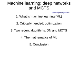
1. Machine learning: deep networks
and MCTS
olivier.teytaud@inria.fr
1. What is machine learning (ML)
2. Critically needed: optimization
3. Two recent algorithms: DN and MCTS
4. The mathematics of ML
5. Conclusion

2. What is machine learning ?
It's when machines learn :-)
● Learn to recognize, classify, make decisions,
play, speak, translate …
● Can be inductive (from data, using statistics)
and/or deductive

3. Examples
● Learn to play chess
● Learn to translate French → English
● Learn to recognize bears / planes / …
● Learn to drive a car (from examples ?)
● Learn to recognize handwritten digits
● Learn which ads you like
● Learn to recognize musics

4. Different flavors of learning
● From data: given 100000 pictures of bears and 100000 pictures
of beers, learn to discriminate a picture of bear and a picture of
beer.
● From data, 2: given 10000 pictures (no categories!
“unsupervised”)
– Find categories and classify
– Or find a “good” representation as a vector
● From simulators: given a simulator (~ the rules) of Chess, play
(well) chess.
● From experience: control a robot, and avoid bumps.
Deductive: not much... (was important at the time of your
grandfathers/grandmothers)

5. Machine learning everywhere ! ! !
Finding ads most likely to get your money.
Local weather forecasts.
Translation.
Handwritten text recognition.
Predicting traffic.
Detecting spam.
...

6. 2. Optimization: a key component of
ML
● Given: a function k: w → k(w)
● Output: w* such that k(w*) minimum
Usually, only an approximation of w*.
Many algorithms exist; one of the best for ML is
stochastic gradient descent.

7. 2.a. Gradient descent
● w = random
● for m=1,2,3,....
– alpha = 0.01 / square-root(m)
– compute the gradient g of k at w
– w = w – alpha g
Key problem: computing g quickly.

8. 2.b. Stochastic gradient descent
● k(w) = k1(w) + k2(w) + … + kn(w)
● Then at iteration i, use the gradient of kj where j=i mod n
==> THE key algorithm for machine learning
● w = random
● for m=1,2,3,....
– Alpha = 0.01 / square-root(m)
– compute the gradient g of k(m mod n) at w
– w = w – alpha g
Gradient can often be computed by “reverse-mode differentiation”, termed
“backpropagation” in neural networks (not that hard)

9. 3. Two ML algorithms
● Part 1: Deep learning (learning to predict)
– Neural networks
– Empirical risk minimization & variants
– Deep networks
● Part 2: MCTS (learning to play)

10. Neuron
x1
x2
x3
z= σ(z)=
w.(x,1) σ(w.(x,1))
1
linear nonlinear
(usually, we do not write the link to “1”)
Formally:
Output=σ(w.(input,1))
w1
w4
w2
w3

11. Neural networks
f(x,w)=σ(w1.x+w1b) w=(w1,w1b)
(==> matrix notations for short: x=vector, w1=matrix, w1b=vector)
X
f(x,w)

12. Neural networks
f(x,w)=σ(w1.x+w1b) w=(w1,w1b)
f(x,w)=σ(w2.σ(w1.x+w1b)+w2b)
w=(w1,w2,w1b,w2b)
X f(x,w)

13. Neural networks
f(x,w)=σ(w1.x+w1b) w=(w1,w1b)
f(x,w)=σ(w2.σ(w1.x+w1b)+w2b) (( =σ(w2.σ(w1x)) ))
w=(w1,w2,w1b,w2b)
f(x,w)= ….. more layers ….
X f(x,w)

14. Neural networks & empirical risk
minimization
Define the model:
f(x,w)=σ(w1.x+w1b) w=(w1,w1b)
f(x,w)=σ(w2.σ(w1.x+w1b)+w2b)
w=(w1,w2,w1b,w2b)
f(x,w)= ….. more layers ….
how to find a good w ?

15. What is a good w ?
Try to find w such that ||f(xi,w) – yi||2
is small
==> finding a predictor of y, given x
X f(x,w)

16. Neural networks & empirical risk
minimization
● Inputs = x1,...,xN (vectors in R^d) and y1,...,yN (vectors in R^k)
● Assumption: the (xi,yi) are randomly drawn, i.i.d, for some probability
distribution
● Define a loss:
L(w) = ( E f(x,w)-y)2
and
its approximation L'(w)= average of (f(x(i),w)-y(i))2
● Optimize:
– Computing w= argmin L(w) impossible (L unknown)
– So w = argmin L'(w) ==> by stochastic gradient descent: gradient ?
Empirical risk

17. Neural networks with SGD
(stochastic gradient descent)
Minimize the sum of the ||f(xi,w) – yi||2
by
●
w ←w – alpha grad ||f(x1,w) – y1||2
●
w ←w – alpha grad ||f(x2,w) – y2||2
● …
●
w ←w – alpha grad ||f(xn,w) – yn||2
● +restart
X f(x,w) ~ y
The network sees
“xi” and “yi”
one at a time.

18. Backpropagation ==> gradient
(thanks http://slideplayer.com/slide/5214241)
● Sigmoid function:
● Partial derivative written in terms of outputs (o)
and activation (z); using derivatives/z (δ)
output node: internal node:

19. Neural networks as encoders
Try to find w such that ||f(xi,w) – xi||2
is small + remove the end
==> finding an encoder of x!
i.e. we get a function f such that x should be a g(f(x)) (for some g).
… looks crazy ? Just f(x)=x is a solution!
X f(x,w)
Delete this ! ! !

20. Ok, neural networks
We have seen two possibilities:
● Neural networks as predictors (supervised)
● Neural networks as encoders (unsupervised)
Both use stochastic gradient descent and ERM.
Now, let us come back to predictors, but with a
better algorithm, for “deep” learning – using
encoders.
From
examples
One example at
a time

21. Empirical risk minimization and
numerical optimization
● We would like to optimize the “real” error (expectation; termed
generalization error, GE) but we have only access to the empirical error
(ER).
● For the same ER, we can have different GE.
● Two questions:
– How to reduce the difference between ER and GE ?
Regularization: minim L'+||w||2 Sparsity: minim L'+||w||0
(small parameters) (few parameters)
==> VC theory (no details here)
– Which of the ER optima are best for GE ? ? ? ?
(now known to be an excellent question!)
==> deep network learning by unsupervised tools!

22. Deep neural networks
● What if many layers ?
● Many local minima (proof: symmetries!)
==> does not work
● Two steps:
– unsupervised learning, layer by layer; the network is
growing;
– then, apply ERM for fine tuning.
● Unsupervised pretraining ==> with the same
empirical error, generalization error is better!

23. Deep networks pretraining
x
x
Train, auto-encoding

24. Deep networks pretraining
This part is learnt.
x

25. Deep networks pretraining
This part is learnt.
x
z
z
Autoencoding!

26. Deep networks pretraining
This part is learnt.
Autoencoding!

27. Deep networks pretraining
Then the network grows!

28. Deep networks pretraining
Then the network grows!

29. Deep networks: supervised!
Learn (supervised learning) the last layer.
x
y

30. Deep networks: supervised!
Learn (supervised learning) the whole network
(fine tuning).
x
y

31. Deep networks in one slide
● For i = 1, 2, 3, …, k:
– Learn one layer by autoencoding (unsupervised)
– Remove the second part
● Learn one more layer in a supervised manner
● Learn the whole network (supervised as well;
fine tuning)

32. Deep networks
● A revolution in vision
● Important point (not developped here): sharing some parameters,
because first layers = low level feature extractors, and LLF are
the same everywhere ==> convolutional nets
● Link with natural learning: learn simple concepts first;
unsupervised learning.
● Not only “σ”, this was just an example;
output=w0.exp(-w2.||input-w1||2)
● Great success in speech & vision
● Surprising performance in Go (discuss later :-) )

33. Part 2: MCTS
● MCTS originates in 2006
● UCT = one particular flavor, from 2007, most
well known probably
● A revolution in Computer Go

34. Part I : The Success Story
(less showing off in part II :-) )
The game of Go is a beautiful
Challenge.

35. Part I : The Success Story
(less showing off in part II :-) )
The game of Go is a beautiful
challenge.
We did the first wins against
professional players
in the game of Go
But with handicap!

36. Game of Go (9x9 here)

37. Game of Go

38. Game of Go

39. Game of Go

40. Game of Go

41. Game of Go

42. Game of Go

43. Game of Go: counting territories
( w h i t e h a s 7 . 5 “ b o n u s ” a s b l a c k s t a r t s )

44. Game of Go: the rules
Black plays at the blue circle:
the white group dies (it is
removed)
It's impossible to kill white (two “eyes”).
“Superko” rule: we don't come back to the same
situation.
(without superko: “PSPACE hard”
with superko: “EXPTIME-hard”)
At the end, we count territories
==> black starts, so +7.5 for white.

45. The rank of MCTS and classical programs in Go
(Source: Peter Shotwell+computer Go mailing list )
Stagnation
around 5D ?
MCTS
RAVE
MPI-parallelization
ML+
Expertise, ...
Quasi-solving
of 7x7
Not over
in 9x9...Alpha
beta

46. MCTS part 2: the UCT algorithm
● MCTS means “Monte Carlo Tree Search”
● UCT means “Upper Confidence Trees”

47. Coulom (06)
Chaslot, Saito & Bouzy (06)
Kocsis Szepesvari (06)
UCT (Upper Confidence Trees)
= Monte Carlo
= random part

48. UCT

49. UCT

50. UCT

51. UCT

52. UCT
Kocsis & Szepesvari (06)

53. Exploitation ...

54. Exploitation ...
SCORE =
5/7
+ k.sqrt( log(10)/7 )

55. Exploitation ...
SCORE =
5/7
+ k.sqrt( log(10)/7 )

56. Exploitation ...
SCORE =
5/7
+ k.sqrt( log(10)/7 )

57. ... or exploration ?
SCORE =
0/2
+ k.sqrt( log(10)/2 )

58. UCT in one slide
Great progress in the game of Go and in various other games

59. Why ?
Why “+ square-root( log(...)/ … )” ?
because there are nice maths on this in
completely different settings.
Seriously, no good reason, use whatever
you want :-)

60. Current status ?
MCTS has invaded game applications:
• For games which have a good simulator
(required!)
• For games for which there is no good
evaluation function, i.e. no simple map
“board → probability that black wins”)
Also some hard discrete control tasks.

61. Current status ?
Go ? Humans still much stronger than
computers.
Deep networks: surprisingly good
performance as an evaluation function.
Still performs far worse than best MCTS.
Merging MCTS and deep networks ?

62. Current MCTS research ?
Recent years:
• parallelization
• extrapolation (between branches of the
search)
But most progress = human expertise
and tricks in the random part.

63. 4. The maths of ML
One can find theorems justifying regularization (+||
w||2 or +||w||0), or theorems justifying that deep
networks need less parameters than shallow
networks for approximating some functions.
Still, MCTS and neural networks were born quite
independently of maths.
Still, you need stochastic gradient descent.
Maybe in the future of ML a real progress born in
maths ?

64. Others

65. Random projection ?
● Randomly project your data (linearly or not)
● Learn on these random projections
● Super fast, not that bad

66. Machine learning + encryption
● Statistics on data... without decrypting them
● Critical for applications
– Where we must “know” what you do (predicting
power consumption)
– But we should not know too much (privacy)

67. Simulation-based + data-based
optimization
● Optimization of models = forgets too many features
from the real world
● Optimization of simulators = better
==> technically, optimization of expensive functions
(the optimization algorithm can spend computational
power) + surrogate model (i.e. ML)

68. Distributed collaborative
decision making ?
● Power network:
– frequency = 50Hz (deviations ≈ )
– (frequency)' = k x (production – demand) → ≈ 0!
● Too much wind power ==> unstable network
because hard to satisfy “production = demand”
● Solutions ?
– Detect frequency
– Increase/decrease production but also demand

69. Limited
capacity
Typical example of natural monopoly.
Deregulation + more distributed production
+ more renewable energy
==> who regulates the network ?
More regulation after all ?
Distributed collaborative decision making.
Ramping
Constraint
(power output
smooth)
IMHO,
Distributed collaborative
decision making is a great
research area (useful + not well
understood)

70. Power systems must change!
● Tired of buying oil which leads to ?
● Don't want ?(coal)
● Afraid of ?
But unstable ?
COME AND HELP ! ! ! STABILIZATION NEEDED :-)

71. Conclusions 1: recent
success stories
● MCTS success story
– 2006: immediately reasonably good
– 2007: thanks to fun tricks in the MC part, strong against pros in
9x9
– 2008: with parallelization, good in 19x19
● Deep networks
– Convolutional DN excellent in 1998 (!) in vision, slightly
overlooked for years
– Now widely recognized in many areas
● Both make sense only with strong computers

72. Conclusions 2: mathematics &
publication & research
● During so many years:
– SVM was the big boss of supervised ML (because there were
theorems, where as there are few theorems in deep learning)
– Alpha-beta was the big boss of games
● MCTS was immediately recognized as a key contribution
to ML; why wasn't it the case for deep learning ? Maybe
because SVM were easier to explain, prove, adverstise.
(but highest impact factor = +squareRoot(... / … ) ! )
● Both deep learning and MCTS look like fun exercises
rather than science; still, they are key tools for ML.
==> keep time for “fun” research, don't worry too much for
publications

73. Conclusions 3: applications are fun!
(important ones :-) )
● Both deep learning and Mcts were born from
applications
● Machine learning came from xps more than
from pure theory
● Automatic driving, micro-emotions (big
brother ?), bioinformatics, …. and POWER
SYSTEMS (with open source / open data!).

74. References
● Backpropagation, Rummelhart et al 1986
● MCTS, Coulom 2006 + Kocsis et al 2007 +
Gelly et al 2007
● Conv. Networks Fukushima 1980
● Deep conv. networks Le Cun 1998
● Regularization, Vapnik et al 1971