Downloaded 1,133 times
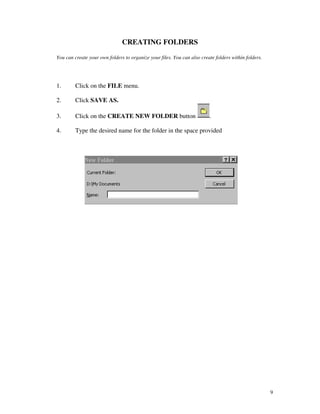
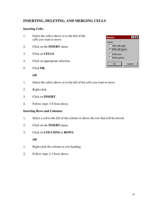
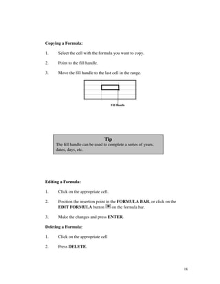
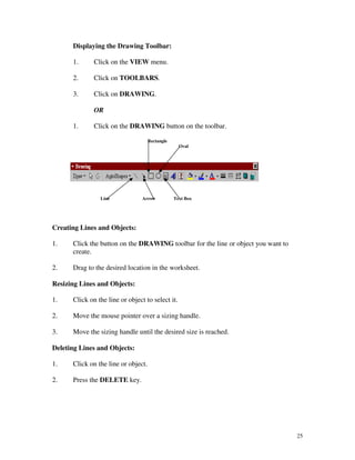
![NAVIGATING THROUGH A WORKSHEET
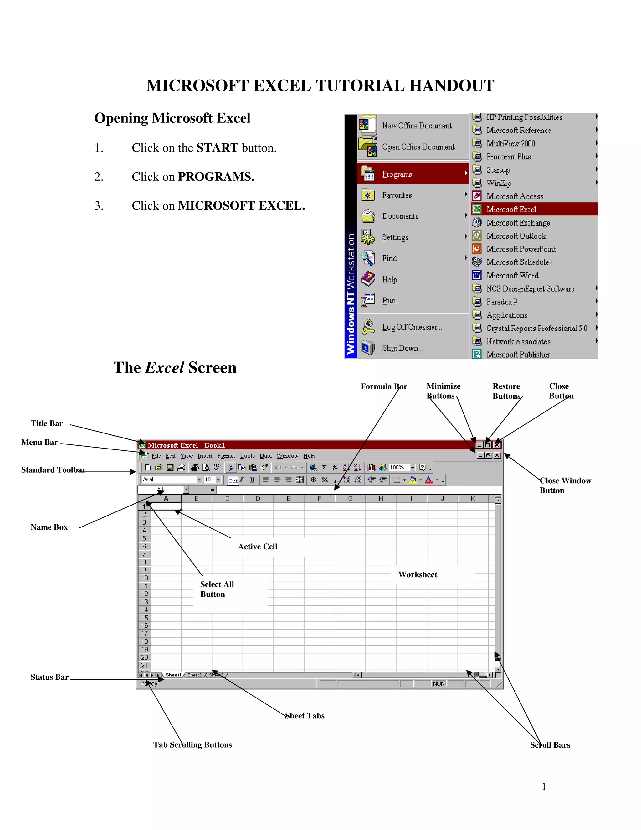
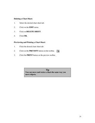
TO MOVE PRESS
Left one column [ ] or Shift + Tab
Right one column [ ] or Tab
To the first column in the worksheet [Ctrl] [ ]
To the last column in the worksheet [Ctrl] [ ]
To the last column in the row with data [Ctrl] [ ]
To the first column in the row with data [Ctrl] [ ]
Up one row [ ] or Shift + Enter
Down one row [ ] or Enter
To the next worksheet Page [Ctrl] [Page Down]
To the previous worksheet Page [Ctrl] [Page Up]
Up one screen [Page Up]
Down one screen [Page Down]
Beginning of worksheet [Ctrl] [Home]
To the last cell with data [Ctrl] [End]
Left one screen [Alt] [Page Up]
Right One Screen [Alt] [Page Down]
4](https://image.slidesharecdn.com/msexceltutorials-100219214739-phpapp01/85/Ms-Excel-Tutorials-4-320.jpg)
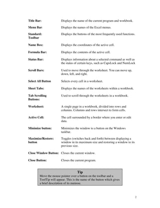
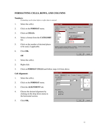
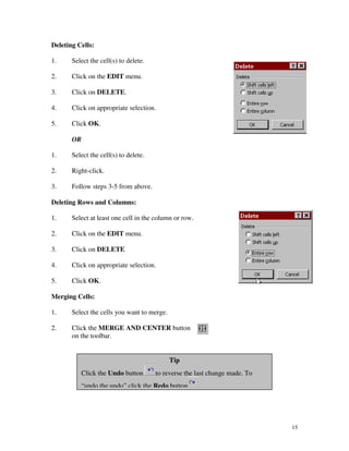
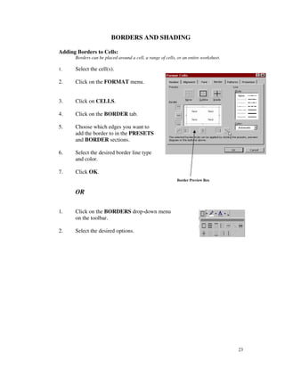
![SAVING A DOCUMENT
Use SAVE AS: when you are saving a new document and you need to name it or if you are opening a
document and saving it with a new name. This does not replace the old file.
Use SAVE: when you are saving changes made to an existing document. The old information will be
overwritten.
Save As:
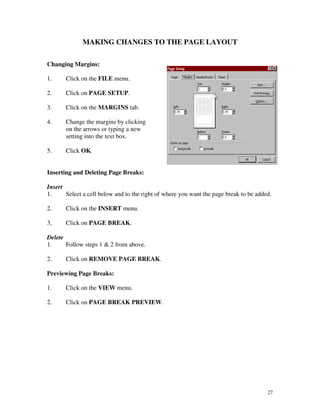
1. Click the FILE menu.
2. Click SAVE AS.
3. Click on the SAVE IN drop down list to select the drive and folder where you
wish to save this document.
4. In the FILE NAME text box, type in the name you wish to give this document.
5. Select “Microsoft Excel Workbook” from the FILE TYPE text box.
6. Click SAVE
Save:
1. Use the SAVE button or press [Ctrl] [S]
10](https://image.slidesharecdn.com/msexceltutorials-100219214739-phpapp01/85/Ms-Excel-Tutorials-10-320.jpg)
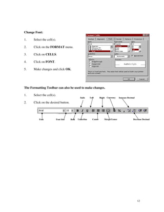
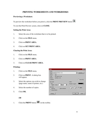
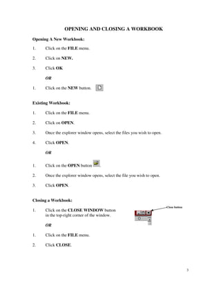
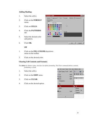
![FIND AND REPLACE
Find:
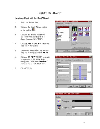
1. Go to the beginning of the document
by pressing [Ctrl] [Home].
2. Click on the EDIT menu.
3. Click on FIND.
4. Click on the FIND tab in the dialog
box that opens.
5. Enter the word or number you wish to find in the “FIND WHAT” text
box.
6. Click on the SEARCH drop-down menu and click on rows or columns.
7. Click on the LOOK IN drop-down menu and click on formulas, values,
or comments.
8. Click on FIND NEXT.
9. Click OK when finished.
21](https://image.slidesharecdn.com/msexceltutorials-100219214739-phpapp01/85/Ms-Excel-Tutorials-21-320.jpg)
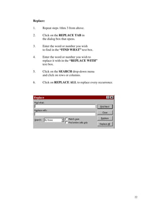

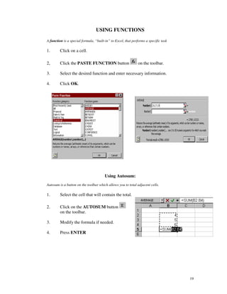
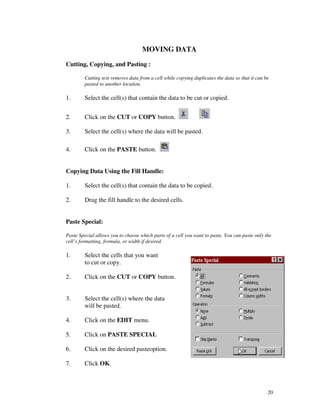
This Excel tutorial document provides instructions on how to perform common tasks in Microsoft Excel, including: 1) Opening and closing workbooks, navigating through worksheets, selecting cells, entering and formatting data, inserting and deleting cells and rows/columns, printing, creating formulas, using functions, moving data, finding and replacing values, and adding borders and shading. 2) It describes the main parts of the Excel interface such as the title bar, menu bar, toolbar, worksheet, scroll bars, and sheet tabs. 3) Step-by-step instructions are provided for common tasks with an emphasis on selecting options from drop-down menus or using keyboard shortcuts for efficient navigation and editing.