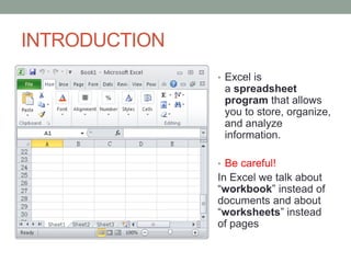
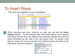
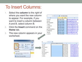
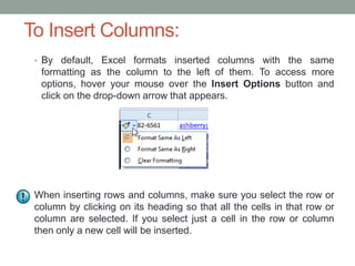
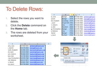
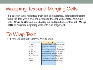
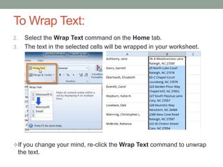
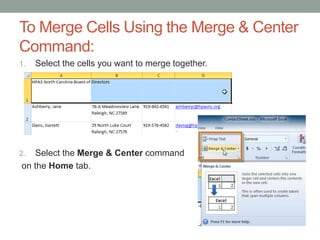
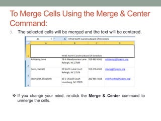
3. INTRODUCTION
• Excel is
a spreadsheet
program that allows
you to store, organize,
and analyze
information.
• Be careful!
In Excel we talk about
“workbook” instead of
documents and about
“worksheets” instead
of pages
7. Create a New Workbook
1. Click the File tab. This takes
you to Backstage view.
2. Select New.
3. Select Blank
workbook under Available
Templates. It will be highlighted
by default.
4. Click Create. A new, blank
workbook appears in the Excel
window.
8. Open an existing Workbook
1. Click the File tab. This takes you
to Backstage view.
2. Select Open. The Open dialog
box appears.
3. Select your desired workbook and
then click Open.
9. Create and open workbooks
• You can see the following video in case you have any
trouble to create or open workbooks
11. The cell
• This video is a good short of the main contents of this
section (cell basics)
12. The cell • Each cell has a name, or a cell
address based on which column
• Each rectangle in a worksheet is and row it intersects. The cell
called a cell. A cell is the address of a selected cell appears
intersection of a row and a column in the Name box. Here you can see
that C5 is selected.
.
13. To select a cell
1. Click on a cell to select it. When a cell is selected you
will notice that the borders of the cell appear bold and
the column heading and row heading of the cell are
highlighted.
2. Release your mouse. The cell will stay selected until
you click on another cell in the worksheet.
3. You can also navigate through your worksheet and
select a cell by using the arrow keys on your keyboard.
14. To Select Multiple Cells:
1. Click and drag your mouse until all of the adjoining
cells you want are highlighted.
2. Release your mouse. The cells will stay selected until
you click on another cell in the worksheet.
15. To Insert Content:
1. Click on a cell to select it.
2. Enter content into the selected cell using your keyboard. The
content appears in the cell and in the formula bar. You also
can enter or edit cell content from the formula bar.
16. To Delete Content Within Cells:
1. Select the cells which contain content you want to delete.
2. Click the Clear command on the ribbon. A dialog box will
appear.
3. Select Clear Contents.
You can also use your
keyboard's Backspace
key to delete content
from a single
cell or Delete key to
delete content
from multiple cells.
17. To Delete Cells:
1. Select the cells that you want to delete.
2. Choose the Delete command from the ribbon.
There is an important difference between deleting the content of a
cell and deleting the cell itself. If you delete the cell, by default the
cells underneath it will shift up and replace the deleted cell.
18. To Copy (or cut) and Paste Cell Content:
1. Select the cells you wish to copy/cut.
2. Click the Copy/cut command. The border of the selected cells
will change appearance.
3. Select the cell or cells where you want to paste the content.
4. Click the Paste command. The copied content will be entered into
the highlighted cells.
19. To Access More Paste Options:
• There are more Paste options
that you can access from the
drop-down menu on
the Paste command. These
options may be convenient to
users who are working
with cells that contain
formulas or formatting.
20. To Access Formatting Commands by
Right-Clicking:
1. Select the cells you
want to format.
2. Right-click on the
selected cells.
A dialog box will
appear where you
can easily access
many commands
that are on the
ribbon.
21. To Drag and Drop Cells:
1. Select the cells that you wish to move.
2. Position your mouse on one of the outside edges of the selected
cells. The mouse changes from a white cross to a black cross
with 4 arrows.
1. Click and drag the cells to the new location.
2. Release your mouse and the cells will be dropped there.
22. To Use the Fill Handle to Fill Cells:
1. Select the cell or cells containing the content you want to use. You
can fill cell content either vertically or horizontally.
2. Position your mouse over the fill handle so that the white
cross becomes a black cross.
3. Click and drag the fill handle until all the cells you want to fill
are highlighted.
4. Release the mouse and your cells will be filled.
23. First challenge!
• Open the document “Exercise1.xls” and do the necessary
modifications to get the next table:
Save as “Ex1_group_your names.xls” and send it to vanesa.rey@sek.es.
25. Working with cells, rows and columns
• This video is a good short of the main contents of this
section:
26. To Modify Column Width:
1. Position your mouse over the column line in the column
heading so that the white cross becomes a double arrow .
2. Click and drag the column to the right to increase the column
width or to the left to decrease the column
3. Release the mouse. The column width will be changed in your
spreadsheet.
27. To Set Column Width with a Specific
Measurement:
1. Select the columns you want to
modify.
2. Click the Format command on the
Home tab. The format drop-down
menu appears.
3. Select Column Width.
4. The Column Width dialog box
appears. Enter a specific
measurement.
5. Click OK. The width of each
selected column will be changed in
your worksheet.
Select AutoFit Column Width from
the format drop-down menu and Excel
will automatically adjust each selected
column so that all the text will fit.
28. To Modify the Row Height:
1. Position the cursor over
the row line so that the
white cross becomes a
double arrow .
2. Click and drag the row
downward to increase the
row height or upward
decrease the row height.
3. Release the mouse. The
height of each selected
row will be changed in
your worksheet.
29. To Set Row Height with a Specific
Measurement:
1. Select the rows you want to modify.
2. Click the Format command on the Home
tab. The format drop-down menu
appears.
3. Select Row Height.
4. The Row Height dialog box appears.
Enter a specific measurement
5. Click OK. The selected rows heights will
be changed in your spreadsheet.
Select AutoFit Row Height from the
format drop-down menu and Excel will
automatically adjust each selected row so
that all the text will fit.
30. To Insert Rows:
1. Select the row below where you want the new row to appear.
2. Click the Insert command on the Home tab.
.
31. To Insert Rows
3. The new row appears in your worksheet
When inserting new rows, columns, or cells, you will see the Insert
Options button by the inserted cells. This button allows you to choose
how Excel formats them. By default, Excel formats inserted rows with the
same formatting as the cells in the row above them. To access more
options, hover your mouse over the Insert Options button and click on the
drop-down arrow that appears.
32. To Insert Columns:
1. Select the column to the right of
where you want the new column
to appear. For example, if you
want to insert a column between
A and B, select column B.
2. Click the Insert command on the
Home tab.
3. The new column appears in your
worksheet.
33. To Insert Columns:
• By default, Excel formats inserted columns with the same
formatting as the column to the left of them. To access more
options, hover your mouse over the Insert Options button and
click on the drop-down arrow that appears.
When inserting rows and columns, make sure you select the row or
column by clicking on its heading so that all the cells in that row or
column are selected. If you select just a cell in the row or column
then only a new cell will be inserted.
34. To Delete Rows:
1. Select the rows you want to
delete.
2. Click the Delete command on
the Home tab.
3. The rows are deleted from your
worksheet.
35. Wrapping Text and Merging Cells
• If a cell contains more text than can be displayed, you can choose to
wrap the text within the cell or merge the cell with empty, adjoining
cells. Wrap text to make it display on multiple lines of the cell. Merge
cells to combine adjoining cells into one larger cell.
To Wrap Text:
1. Select the cells with text you want to wrap.
36. To Wrap Text:
2. Select the Wrap Text command on the Home tab.
3. The text in the selected cells will be wrapped in your worksheet.
If you change your mind, re-click the Wrap Text command to unwrap
the text.
37. To Merge Cells Using the Merge & Center
Command:
1. Select the cells you want to merge together.
2. Select the Merge & Center command
on the Home tab.
38. To Merge Cells Using the Merge & Center
Command:
3. The selected cells will be merged and the text will be centered.
If you change your mind, re-click the Merge & Center command to
unmerge the cells.
39. To Access More Merge Options:
Click the drop-down arrow next to the Merge & Center command on
the Home tab. The merge drop-down menu appears.
• Merge & Center: Merges selected cells into one cell and centers the
text.
• Merge Across: Merges each row of selected cells into larger cells.
This command is useful if you are merging content across multiple
rows of cells and do not want to create one large cell.
• Merge Cells: Merges selected cells into one cell.
• Unmerge Cells: Unmerges the selected cells.
41. FORMATTING TEXT
• Watch the video to learn how to use Font, Alignment, and
Number commands to format text in an Excel 2010
workbook.
More information: http://www.gcflearnfree.org/excel2010/4.1
42. Second challenge!
Arial 14 (bold/underline)
Row height: 40
Calibri 12 (bold)
• Open your previous
exercise (first challenge)
and convert it into this
table.
• Save as
Calibri
10 “Ex2_group_your
names.xls” and send it to
vanesa.rey@sek.es
Italic
Column
height:16
44. WORKSHEETS
• When you open an Excel workbook, there are three worksheets by
default. The default names on the worksheet tabs are Sheet1,
Sheet2 and Sheet3. To organize your workbook and make it easier to
navigate, you can rename and even color-code the worksheet tabs.
Additionally, you can insert, delete, move, and copy worksheets.
• Watch the video to learn about worksheets.
• More information: http://www.gcflearnfree.org/excel2010/7.2
45. Third challenge!
• Open the document “Exercise3.xls”.
• Change the names of the three worksheets:
Sheet1- January
Sheet2- March
Sheet3- February
• Move the worksheets to put the months in order.
• Add a new sheet. Its name has to be “april”.
• The Color-Code for Worksheet Tabs has to be:
January- red February- green
March – purple April – blue
• Save as “Ex3_group_your names.xls” and send it to
vanesa.rey@sek.es.