Download as PPS, PPTX
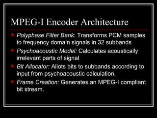
![MPEG-I Encoder Architecture[1]](https://image.slidesharecdn.com/pan95gakhal-160522003928/85/MPEG-Audio-Compression-7-320.jpg)
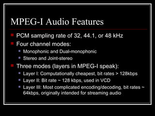
![Polyphase Filter Bank
Divides audio signal into 32 equal width
subband streams in the frequency domain.
Inverse filter at decoder cannot recover
signal without some, albeit inaudible, loss.
Based on work by Rothweiler[2].
Standard specifies 512 coefficient analysis
window, C[n]](https://image.slidesharecdn.com/pan95gakhal-160522003928/85/MPEG-Audio-Compression-10-320.jpg)
![Polyphase Filter Bank
Buffer of 512 PCM samples with 32 new
samples, X[n], shifted in every computation cycle
Calculate window samples for i=0…511:
Partial calculation for i=0…63:
Calculate 32 subsamples:
][][][ iXiCiZ ⋅=
∑=
+=
7
0
]64[][
j
jiZiY
∑=
⋅=
63
0
]][[][][
k
kiMiYiS](https://image.slidesharecdn.com/pan95gakhal-160522003928/85/MPEG-Audio-Compression-11-320.jpg)
![Polyphase Filter Bank
Visualization of the filter[1]
:](https://image.slidesharecdn.com/pan95gakhal-160522003928/85/MPEG-Audio-Compression-12-320.jpg)
![Polyphase Filter Bank
The net effect:
Analysis matrix:
Requires 512 + 32x64 = 2560 multiplies.
Each subband has bandwidth π/32T centered at
odd multiples of π/64T
]64[]64[]][[][
63
0
7
0
jiXjiCkiMiS
k j
++= ∑ ∑= =
−+
=
64
)16)(12(
cos]][[
πki
kiM](https://image.slidesharecdn.com/pan95gakhal-160522003928/85/MPEG-Audio-Compression-13-320.jpg)
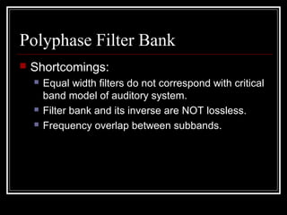
![Polyphase Filter Bank
Comparison of filter banks and critical bands[1]:](https://image.slidesharecdn.com/pan95gakhal-160522003928/85/MPEG-Audio-Compression-15-320.jpg)
![Polyphase Filter Bank
Frequency response of one subband[1]
:](https://image.slidesharecdn.com/pan95gakhal-160522003928/85/MPEG-Audio-Compression-16-320.jpg)
![Psychoacoustic Model (example)
Input[1]
:](https://image.slidesharecdn.com/pan95gakhal-160522003928/85/MPEG-Audio-Compression-25-320.jpg)
![Psychoacoustic Model (example)
Transformation to perceptual domain[1]
:](https://image.slidesharecdn.com/pan95gakhal-160522003928/85/MPEG-Audio-Compression-26-320.jpg)
![Psychoacoustic Model (example)
Calculation of masking thresholds[1]
:](https://image.slidesharecdn.com/pan95gakhal-160522003928/85/MPEG-Audio-Compression-27-320.jpg)
![Psychoacoustic Model (example)
Signal-to-mask ratios[1]
:](https://image.slidesharecdn.com/pan95gakhal-160522003928/85/MPEG-Audio-Compression-28-320.jpg)
![Psychoacoustic Model (example)
What we actually send[1]
:](https://image.slidesharecdn.com/pan95gakhal-160522003928/85/MPEG-Audio-Compression-29-320.jpg)
![Layer Specific Coding
Layer specific frame formats[1]
:](https://image.slidesharecdn.com/pan95gakhal-160522003928/85/MPEG-Audio-Compression-31-320.jpg)
![Layer Specific Coding
Stream of samples is processed in groups[1]
:](https://image.slidesharecdn.com/pan95gakhal-160522003928/85/MPEG-Audio-Compression-32-320.jpg)
![References
[1] D. Pan, “A Tutorial on MPEG/Audio Compression”,
IEEE Multimedia Journal, 1995.
[2] J. H. Rothweiler, “Polyphase Quadrature Filters – a New
Subband Coding Technique”, Proc of the Int. Conf. IEEE
ASSP, 27.2, pp1280-1283, Boston 1983.](https://image.slidesharecdn.com/pan95gakhal-160522003928/85/MPEG-Audio-Compression-41-320.jpg)

This document provides an overview of MPEG-1 audio compression. It describes the key components of the MPEG-1 audio encoder including the polyphase filter bank that transforms audio into frequency subbands, the psychoacoustic model that determines inaudible parts of the signal, and the coding and bit allocation process that assigns bits to subbands. The overview concludes by noting that MPEG-1 audio provides high compression while retaining quality and paved the way for future audio compression standards.