Download as PDF, PPTX
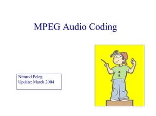

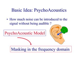
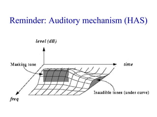
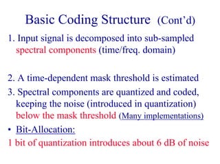
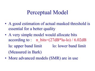
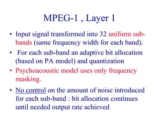
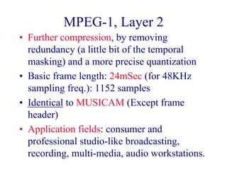
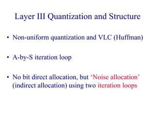
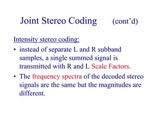
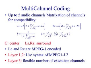
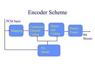
![Non-Linear Critical Bands
0 2 4 6 8 10 12 14 16 18 20 22 24
0 3 6 9 12 15
Critical Bands [KHz]
Bark Numbers](https://image.slidesharecdn.com/a1mpeg12-2004-180403020133/85/A1mpeg12-2004-32-320.jpg)
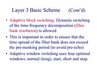
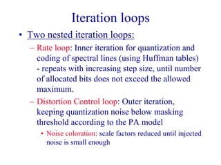
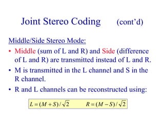
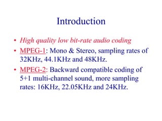
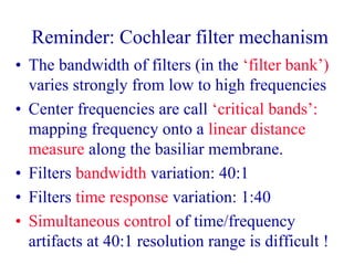
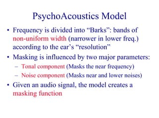
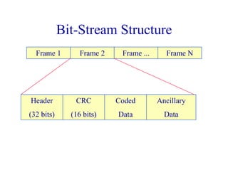
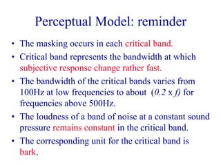
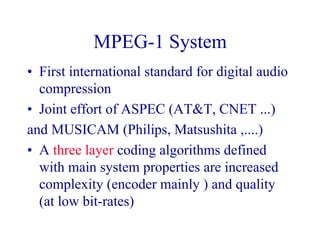
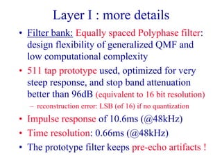
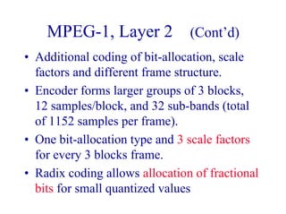
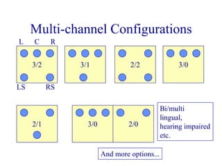
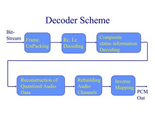
![PA Model I (Cont’d)
• Global masking threshold, LTg, (for the
frequency component) is derived by
summing the powers of the individual
masking thresholds (tonal: LTtm , non-tonal LTnm )
and the threshold in quite:
[dB]101010log10)(
1
10/),(
1
10/),(10/)(
10
++= ∑∑ ==
n
j
ijLTnm
m
j
ijLTtmiLTq
iLTg](https://image.slidesharecdn.com/a1mpeg12-2004-180403020133/85/A1mpeg12-2004-48-320.jpg)
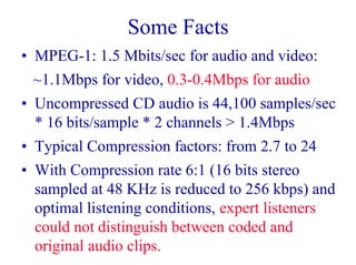
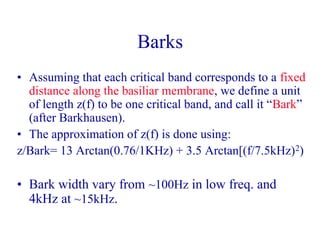
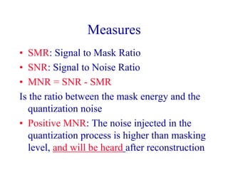
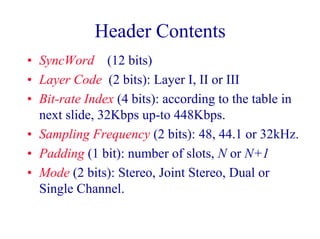
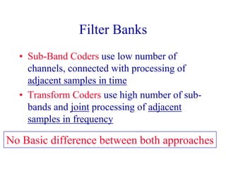
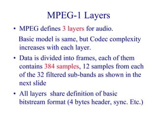
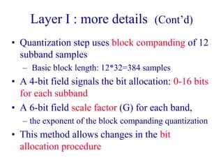
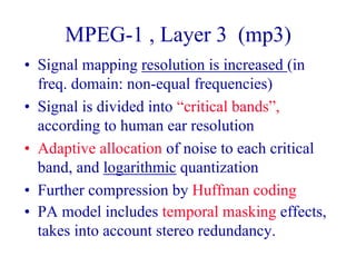
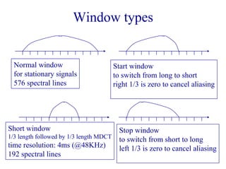
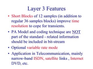
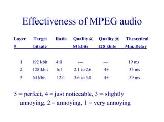
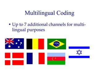
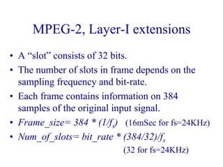
![PA Model I (Cont’d)
• To determine the Signal-to-Mask Ratio
(SMR) in sub-band n, the minimum global
masking threshold LTmin is used:
[dB])()()( min nLTnLnSMR SBSB −=
Where LSB(n) is the signal component
in sub-band n .](https://image.slidesharecdn.com/a1mpeg12-2004-180403020133/85/A1mpeg12-2004-49-320.jpg)
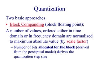
![PA Model II (Cont’d)
• SMR is calculated by the ratio between
energy in the “scale factor” band (e_partn)
and the noise level in the scale factor band
(n_partn):
[dB])_/_(log10 10 nnn partnparteSMR =
n: index of coder partition
Scale factor: the maximum of the absolute values of 12 samples in
a sub-band is determined. (6 bits)](https://image.slidesharecdn.com/a1mpeg12-2004-180403020133/85/A1mpeg12-2004-51-320.jpg)
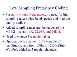
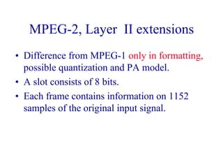
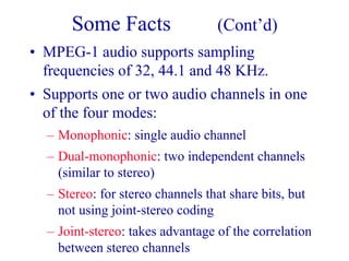
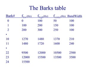
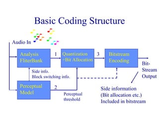
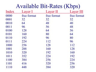
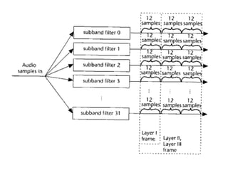
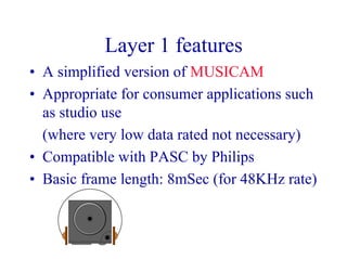
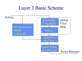
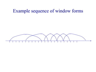
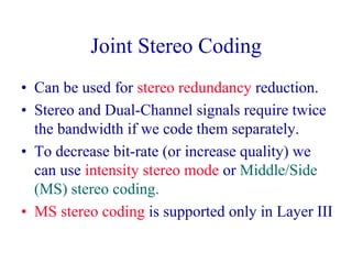
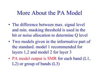
![Witches:Witches: ““DingoDingo”” at 22.05Khzat 22.05Khz
0
10
20
30
40
50
60
70
80
90
100
128 112 96 80 64 56 48 40 32 24 16
bitrate [KBits/sec]
0
5
10
15
20
25
quality [4.5-5] quality [3.5-4.5] quality [2.5-3.5] quality [1.5-2.5] quality [1-1.5] SNR [dB]
Successful
granules SNR](https://image.slidesharecdn.com/a1mpeg12-2004-180403020133/85/A1mpeg12-2004-62-320.jpg)

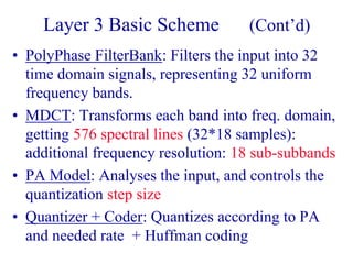
The document discusses MPEG audio coding standards. Key points: - MPEG-1 and MPEG-2 standards support audio compression for low bitrate streaming. MPEG-1 supports mono, stereo up to 48KHz. MPEG-2 adds support for 5.1 surround sound and lower sampling rates. - Layer 1 is a basic implementation while Layers 2 and 3 provide increased compression using psychoacoustic models and more advanced quantization techniques. Layer 3 (MP3) is commonly used. - Psychoacoustic models estimate masking thresholds to allow quantization noise below audible levels, improving compression ratios. Critical band models approximate the ear's frequency resolution.


![[Deck] What's New in Spark-Iceberg Integration via DSV2.pptx](https://cdn.slidesharecdn.com/ss_thumbnails/deckwhatsnewinspark-icebergintegrationviadsv2-260210005337-25955b12-thumbnail.jpg?width=640&height=640&fit=bounds)


