This document discusses various media compression techniques including JPEG for images, MP3 and AAC for audio, and MPEG standards for video. JPEG takes advantage of human insensitivity to high spatial frequencies to compress images. MP3 audio compression utilizes properties of human hearing like insensitivity to quiet frequencies. MPEG video standards like H.261 and MPEG-2 achieve higher compression by exploiting both spatial and temporal redundancy between frames.

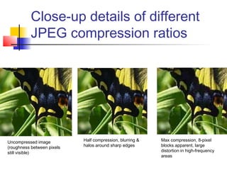
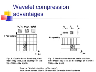
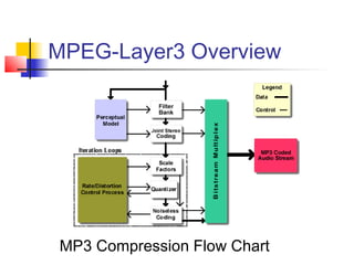
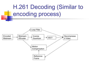
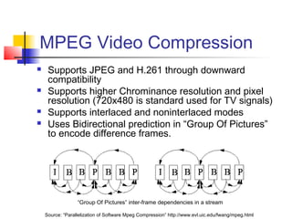
1. Media Compression
Techniques
Michael Moewe
EE290F, Spring 2004
Professor Kaminow

2. Table of Contents
 Image Compression Methods
 JPEG
 GIF 89a
 Wavelet Compression
 Fractal
 Sound Compression
 MPEG Audio Overview
 MPEG Layer-3 (MP3)
 MPEG AAC
 Video Compression Methods
 H.261
 MPEG/MPEG-2
 MPEG-4
 MPEG-7

3. JPEG Compression: Basics
 Human vision is insensitive to high spatial frequencies
 JPEG Takes advantage of this by compressing high frequencies
more coarsely and storing image as frequency data
 JPEG is a “lossy” compression scheme.
Losslessly compressed image, ~150KB JPEG compressed, ~14KB

4. Digital Image Representation
 JPEG can handle arbitrary color spaces
(RGB, CMYK, YCbCr (separates colors into
grayscale components)
 Luminance/Chrominance commonly used,
with Chrominance subsampled due to human
vision insensitivity
 Uncompressed spatial color data components
are stored in quantized values (8, 16, 24bit,
etc).

5. Flow Chart of JPEG
Compression Process
 Divide image into 8x8 pixel blocks
 Apply 2D Fourier Discrete Cosine Transform
(FDCT) Transform
 Apply coarse quantization to high spatial
frequency components
 Compress resulting data losslessly and store
8x8
pixel
blocks
FDC
T
Frequency
Dependent
quantization
Zig-zag
scan
Huffman
encoding
JPEG
syntax
generator
Quantization
Table
output

6. Example of Frequency
Quantization with 8x8 blocks
128 128 128 128 128 128 128 128
118 111 112 117 120 123 123 122
125 121 115 111 119 119 118 117
120 121 113 113 125 124 115 108
120 120 116 119 124 120 115 110
117 113 111 122 120 110 116 119
109 113 111 122 120 110 116 119
111 121 124 118 115 121 117 113
-80 4 -6 6 2 -2 -2 0
24 -8 8 12 0 0 0 2
10 -4 0 -12 -4 4 4 -2
8 0 -2 -6 10 4 -2 0
18 4 -4 6 -8 -4 0 0
-2 8 6 -4 0 -2 0 0
12 0 6 0 0 0 -2 -2
0 8 0 -4 -2 0 0 0
16 11 10 16 24 40 51 61
12 12 14 19 26 58 60 55
14 13 16 24 40 57 69 56
14 17 22 29 51 87 80 62
18 22 37 56 68 109 103 77
24 35 55 64 81 104 113 92
49 64 78 87 103 121 120 101
72 92 95 98 112 100 103 99
-5 0 0 0 0 0 0 0
2 -1 1 1 0 0 0 0
1 0 0 -1 0 0 0 0
1 0 0 0 0 0 0 0
1 0 0 0 0 0 0 0
0 0 0 0 0 0 0 0
0 0 0 0 0 0 0 0
0 0 0 0 0 0 0 0
Quantization Matrix to divide by
Color space values (spatial data)
Quantized spatial frequency values
Color space values (spatial data)

7. Scanning and Huffman
Encoding
-5 0 0 0 0 0 0 0
2 -1 1 1 0 0 0 0
1 0 0 -1 0 0 0 0
1 0 0 0 0 0 0 0
1 0 0 0 0 0 0 0
0 0 0 0 0 0 0 0
0 0 0 0 0 0 0 0
0 0 0 0 0 0 0 0
 Spatial Frequencies scanned in zig-zag
pattern (note high frequencies mostly zero)
 Huffman encoding used to losslessly record
values in table
0,2,1,-1,0,0,1,0,1,1,0,0,1,0,0,0,-1,0,0,… 0
Can be stored as:
(1,2),(0,1),(0,-1),(2,1),(1,1),(0,1),(0,1),(2,1),(3,1),EOB

8. Examples of varying JPEG
compression ratios
500KB image, minimum compression 40KB image, half compression 11KB image, max compression

9. Close-up details of different
JPEG compression ratios
Uncompressed image
(roughness between pixels
still visible)
Half compression, blurring &
halos around sharp edges
Max compression, 8-pixel
blocks apparent, large
distortion in high-frequency
areas

10. JPEG Encoding modes
 Sequential mode
 Image scanned in a raster scan with single pass, 8-bit
resolution
 Sequential mode
 Step-by-step buildup of image from low to high frequency,
useful for applications with long loading times (internet,
portable devices, etc)
 Hierarchical mode
 Encoded using low spatial resolution image and encoding
higher resolution images based on interpolated difference,
for display on varying equipment

11. GIF 89a Image Compression
 Compuserve’s image compression
format
 Best for images with sharp edges, low
bits per channel, computer graphics
where JPEG spatial averaging is
inadequate
 Usually used with 8-bit images,
whereas JPEG is better for 16-bit
images.

12. GIF 89a examples vs. JPEG
GIF Image, 7.5KB,
optimal encoding
JPEG, blotchy spots in single-
color areas

13. Wavelet Image Compression
 Optimal for images containing
sharp edges, or continuous
curves/lines (fingerprints)
 Compared with DCT, uses
more optimal set of functions
to represent sharp edges
than cosines.
 Wavelets are finite in extent
as opposed to sinusoidal
functions
Several different families of wavelets.
Source: “An Introduction to Wavelets”.
http://www.amara.com/IEEEwave/IEEEwavelet.html#contents

14. Wavelet vs. JPEG
compression
Wavelet compression
file size: 1861 bytes
compression ratio - 105.6
Source: “About Wavelet Compression”. http://www.barrt.ru/parshukov/about.htm.
JPEG compression
file size: 1895 bytes
compression ratio - 103.8

15. Wavelet compression
advantages
Fig. 1. Fourier basis functions, time-
frequency tiles, and coverage of the
time-frequency plane.
Fig. 2. Daubechies wavelet basis functions,
time-frequency tiles, and coverage of the time-
frequency plane
Source: “An Introduction to Wavelets”.
http://www.amara.com/IEEEwave/IEEEwavelet.html#contents

16. Fractal Based Image
Compression
 Image compressed in terms of self-
similarity rather than pixel resolution
 Can be digitally scaled to any resolution
when decoded

17. Table of Contents
 Image Compression Methods
 JPEG
 GIF 89a
 Wavelet Compression
 Fractal
 Sound Compression
 MPEG Audio Overview
 MPEG Layer-3 (MP3)
 MPEG AAC
 Video Compression Methods
 H.261
 MPEG/MPEG-2
 MPEG-4
 MPEG-7

18. MPEG Audio basics &
Psychoacoustic Model
 Human hearing limited to values lower than
~20kHz in most cases
 Human hearing is insensitive to quiet
frequency components to sound
accompanying other stronger frequency
components
 Stereo audio streams contain largely
redundant information
 MPEG audio compression takes advantage of
these facts to reduce extent and detail of
mostly inaudible frequency ranges

19. MPEG-Layer3 Overview
MP3 Compression Flow Chart

20. MPEG Layer-3 performance
sound quality bandwidth mode bitrate reduction ratio
telephone sound 2.5 kHz mono 8 kbps * 96:1
better than short wave 4.5 kHz mono 16 kbps 48:1
better than AM radio 7.5 kHz mono 32 kbps 24:1
similar to FM radio 11 kHz stereo 56...64 kbps 26...24:1
near-CD 15 kHz stereo 96 kbps 16:1
CD >15 kHz stereo 112..128kbps 14..12:1

21. MPEG-2 Advanced Audio Coding
(AAC) codec (next generation)
 Sampling frequencies from 8kHz to 96kHz
 1 to 48 channels per stream
 Temporal Noise Shaping (TNS) smooths
quantization noise by making frequency
domain predictions
 Prediction: Allows predictable sound patterns
such as speech to be predicted and
compressed with better quality

22. MPEG-2 AAC Flowchart

23. Table of Contents
 Image Compression Methods
 JPEG
 GIF 89a
 Wavelet Compression
 Fractal
 Sound Compression
 MPEG Audio Overview
 MPEG Layer-3 (MP3)
 MPEG AAC
 Video Compression Methods
 H.261
 MPEG/MPEG-2
 MPEG-4
 MPEG-7

24. Video Compression with
Temporal Redundancy
 Using strictly spatial redundancy
(JPEG) gives video compression ratios
from 7:1 to 27:1
 Taking advantage of temporal
redundancy in video gives 20:1 to 300:1
compression for H.261, or 30:1 to 100:1
for high quality MPEG-2

25. Videoconferencing
Compression with H.261
 H.261 is standard recommended for
videoconferencing over ISDN lines.
 Takes advantage of both spatial and
temporal redundancy in moving images
 Extremely similar to JPEG, but uses
initial frame plus motion vectors to
predict subsequent frames

26. H.261 Block Structure
 Basic unit of processing is in 8x8 pixel
blocks.
 Macro Blocks (MB, 16x16 pixels) are
used for motion estimation, 4 blocks of
luminance, 2 of chrominance
 Groups of Blocks (GOB) of 3x11 MB’s
are stored together with a header in
stream.

27. H.261 Block Structure of
bitstream
Source: “H.261 Videoconferencing Codec” http://www.uh.edu/~hebert/ece6354/H261-report.pdf
Block structure of H.261 video bitstream, Common Intermediate
Format (CIF), 360x288 pixels luminance, 180x144 pixels chrominance

28. H.261 Decoding (Similar to
encoding process)
Encoded
Bitstream
Bitstream
DEcoder
Loop Filter
Inverse
Quantizer IDCT
Decompresse
d Video
Motion
Compensation
Reference
Frame

29. MPEG Video Compression
 Supports JPEG and H.261 through downward
compatibility
 Supports higher Chrominance resolution and pixel
resolution (720x480 is standard used for TV signals)
 Supports interlaced and noninterlaced modes
 Uses Bidirectional prediction in “Group Of Pictures”
to encode difference frames.
Source: “Parallelization of Software Mpeg Compression” http://www.evl.uic.edu/fwang/mpeg.html
“Group Of Pictures” inter-frame dependencies in a stream

30. MPEG 1 & 2 Bitstream
Source: http://www.doc.ic.ac.uk/~nd/surprise_96/journal/vol4/sab/report.html
The MPEG data hierarchy

31. MPEG-4
 Original goal was for 10 times better
compression than H.261
 Goals shifted to
 Flexible bitstreams for varying receiver capabilities
 Stream can contain new applications and
algorithms
 Content-based interactivity with data stream
 Network independence (used for Internet,
Wireless, POTS, etc)
 Object based representations

32. MPEG-4 audio-visual scene
composition
 Can place media objects anywhere in a
scene
 Apply transforms to change appearance or
qualities of an object
 Group objects to form compound objects
 Apply streamed data to objects
 Interactively change viewer’s position in the
virtual scene
http://www.iis.fraunhofer.de/amm/techinf/mpeg4/mp4_overv.pdf

33. MPEG-4 “Audiovisual Scene”
Example
Source: “MPEG-4 Overview” http://www.chiariglione.org/mpeg/standards/mpeg-4/mpeg-4.htm

34. MPEG-7
 Media tagging format for doing searches on arbitrary media formats via
feature extraction algorithms
 Visual descriptors such as:
 Basic Structures
 Color
 Texture
 Shape
 Localization of spatio-temporal objects
 Motion
 Face Recognition
 Audio descriptors such as :
 Sound effects description
 Musical Instrument Timbre Description
 Spoken Content Description
 Melodic Descriptors (search by tune)
 Uniform Silence Segment
 Example application: Play a few notes on a keyboard and have
matched song retrieved.

35. Conclusion
 Media compression is indispensable
even as storage and streaming
capacities increase
 Future goals oriented towards
increasing ease of access to media
information (similar to google for text
based information)

36. References
 MPEG Overview (
http://www.chiariglione.org/mpeg/standards/mpeg-4/mpeg-4.htm)
 Wu C., Irin J. “Emerging Multimedia Computer Communication Technologies”.
1998, Prentice Hall PTR, NJ.
 Overview of the MPEG-4 Standard (
http://www.iis.fraunhofer.de/amm/techinf/mpeg4/mp4_overv.pdf)
 Digital Video, MPEG and Associated Artifacts (
http://www.doc.ic.ac.uk/~nd/surprise_96/journal/vol4/sab/report.html)
 Parallelization of Software MPEG Compression (
http://www.evl.uic.edu/fwang/mpeg.html)
 H.261 Video Teleconferencing Codec (
http://www.uh.edu/~hebert/ece6354/H261-report.pdf)
 An Introduction to Wavelets (
http://www.amara.com/IEEEwave/IEEEwavelet.html#contents)
 About Wavelet Compression (http://www.barrt.ru/parshukov/about.htm)