Downloaded 41 times


![Performance
Measure
2) Are there holistic objectives that model
choice based upon accuracy might hurt?
Choosing a model to deploy based purely on predictive
power may pose ethical problems. Some examples:
● A risk score algorithm that predicts whether someone
will commit a future crime, used by US courts,
discriminated based upon race. It was clear the model
relied heavily on race as a feature. [Link]
● Carnegie Mellon found that women were less likely
than men to be shown ads by Google for high paying
jobs. [Link]
● Orbitz, a travel site, was showing Mac users higher
priced travel services than PC users. [Link]
We have values
as a society
that are not
captured by
optimizing for
accuracy.](https://image.slidesharecdn.com/module4modelselectionandevaluation2-190707194704/85/Module-4-Model-Selection-and-Evaluation-12-320.jpg)
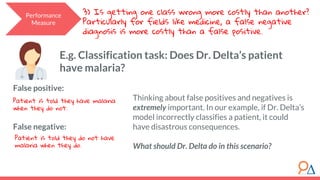
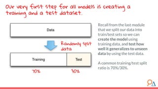


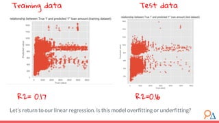
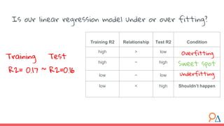

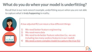
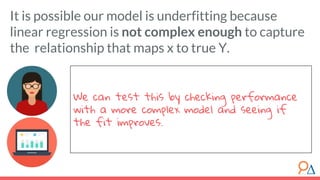
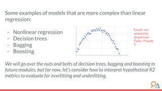

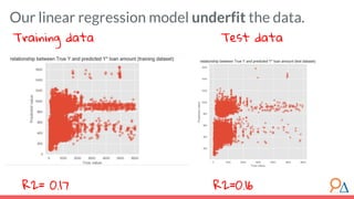
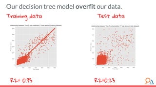
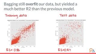
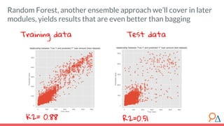
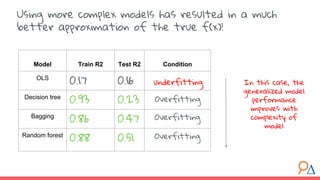
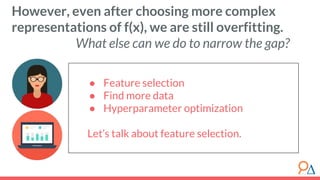


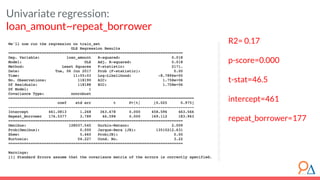

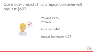
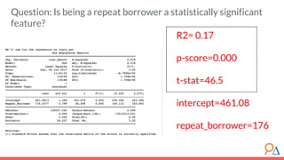
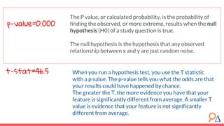


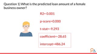
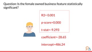


This document outlines a course module on model selection and evaluation, focusing on how to appropriately choose, assess, and validate models in research. It emphasizes the importance of performance measures such as accuracy and mean squared error, as well as considerations regarding ethical implications and generalization to unseen data. Furthermore, the document addresses issues of underfitting and overfitting in model training and suggests methods for improving model performance through feature selection and utilizing more complex algorithms.