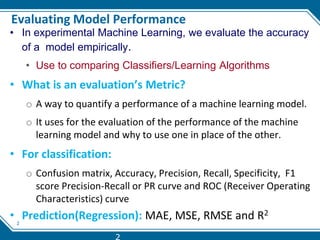
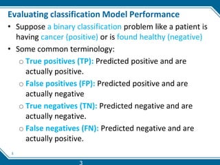
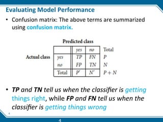
1
ML-Chapter Four:
Model Performance Evaluation
Belay E., Asst. Prof.
e-mail: belayenyew@gmail.com
Mobile: 0946235206
University of Gondar
College of Informatics
Department of Information Technology
2
Evaluating Model Performance
• In experimental Machine Learning, we evaluate the accuracy
of a model empirically.
• Use to comparing Classifiers/Learning Algorithms
• What is an evaluation’s Metric?
o A way to quantify a performance of a machine learning model.
o It uses for the evaluation of the performance of the machine
learning model and why to use one in place of the other.
• For classification:
o Confusion matrix, Accuracy, Precision, Recall, Specificity, F1
score Precision-Recall or PR curve and ROC (Receiver Operating
Characteristics) curve
• Prediction(Regression): MAE, MSE, RMSE and R2
2
3
Evaluating classification Model Performance
• Suppose a binary classification problem like a patient is
having cancer (positive) or is found healthy (negative)
• Some common terminology:
o True positives (TP): Predicted positive and are
actually positive.
o False positives (FP): Predicted positive and are
actually negative
o True negatives (TN): Predicted negative and are
actually negative.
o False negatives (FN): Predicted negative and are
actually positive.
3
4
Evaluating Model Performance
• Confusion matrix: The above terms are summarized
using confusion matrix.
• TP and TN tell us when the classifier is getting
things right, while FP and FN tell us when the
classifier is getting things wrong
4
5
Evaluating Model Performance
• Accuracy (Recognition Rate): calculated as the number
of all correct predictions divided by the total number of
the testing dataset.
o The most commonly used metric to judge a model
o It is not a clear indicator of the performance when classes are
imbalanced.
𝑨𝒄𝒄𝒖𝒓𝒂𝒄𝒚 =
𝑻𝑷 + 𝑻𝑵
𝑻𝑷 + 𝑭𝑷 + 𝑻𝑵 + 𝑭𝑵
• Error rate or misclassification rate:
error rate=1 – accuracy, or
𝒆𝒓𝒓𝒐𝒓 𝒓𝒂𝒕𝒆 =
𝑭𝑷 + 𝑭𝑵
𝑻𝑷 + 𝑭𝑷 + 𝑻𝑵 + 𝑭𝑵
5
6
Example of Confusion Matrix:
• An example of a confusion matrix for the two classes
buys-computer=yes (positive) and buys-computer=no
(negative)
• Accuracy = (TP + TN)/total=(6954+2588)/10000=0.95
• error rate or misclassification rate=1 – accuracy, or
Error rate = (FP + FN)/total=(412+46)/10000=0.05
7
Precision and Recall
• Precision: Percentage of positive instances out of the total
predicted instances i.e., what percentage of tuples labeled as
positive are actually positive.
𝒑𝒓𝒆𝒄𝒊𝒔𝒊𝒐𝒏 =
𝑻𝑷
𝑻𝑷 + 𝑭𝑷
• Recall/Sensitivity/True Positive Rate : Percentage of positive
instances out of the total actual positive instances i.e. what
percentage of positive tuples are labeled as positive.
𝒓𝒆𝒄𝒂𝒍𝒍 𝒐𝒓 𝑻𝑷𝑹 𝒐𝒓 𝒔𝒆𝒏𝒔𝒊𝒕𝒊𝒗𝒊𝒕𝒚 =
𝑻𝑷
𝑻𝑷 + 𝑭𝑵
o Perfect score is 1.0
• Specificity: Percentage of negative instances out of the total actual
negative instances 𝑠𝑝𝑒𝑐𝑖𝑓𝑖𝑐𝑖𝑡𝑦 =
𝑇𝑁
𝑇𝑁+𝐹𝑃
7
8
Precision and Recall-Example
 Based on the previous confusion matrix:
 Precision = 6954/(6954+412) = 0.944 =94.4%
 Recall = 6954/(6954+46)= 0.9934=99.34%
 A perfect precision score of 1.0 for a class C means that
every tuple that the classifier labeled as belonging to class C
does indeed belong to class C. However, it does not tell us
anything about the number of class C tuples that the
classifier mislabeled.
 A perfect recall score of 1.0 for C means that every item
from class C was labeled as such, but it does not tell us how
many other tuples were incorrectly labeled as belonging to
class C
 Specificity=2588/(2588+412)=0.8626=86.26% 8
9
Precision and Recall-Example
F measure (F1 or F-score): harmonic mean of precision and recall.
 It an alternative way to use precision and recall by combining
them into a single measure .
𝑭𝟏 =
𝟐 ∗ 𝒓𝒆𝒄𝒂𝒍𝒍 ∗ 𝒑𝒓𝒆𝒄𝒊𝒔𝒊𝒐𝒏
𝒑𝒓𝒆𝒄𝒊𝒔𝒊𝒐𝒏 + 𝒓𝒆𝒄𝒂𝒍𝒍
F1=(2*0.944*0.9934)/(0.9934+0.944)=1.8755392/1.9374=0.9680
• The higher the F1 score, the better.
Suppose
Model 1: Recall =70% and precision= 60%
Model 2: Recall =80% and precision=50%
Which model is better? Use F measure
10
class imbalance problem
 where the main class of interest is rare.
 The data set distribution reflects a significant majority of the
negative class and a minority of positive class.
• For example, in fraud detection applications, the class of
interest (or positive class) is “fraud,” which occurs much
less frequently than the negative “nonfraudulant” class.
• class imbalance problem identified using:
o Sensitivity is also referred to as the true positive (recognition)
rate (i.e., the proportion of positive tuples that are correctly
identified), while specificity is the true negative rate (i.e., the
proportion of negative tuples that are correctly identified)
10
11
class imbalance problem
Example, a confusion matrix for medical data where the class values are yes and no
for a class label attribute, cancer.
• Confusion matrix for the classes cancer=yes and cancer =no.
 The sensitivity of the classifier is 90/300=30%
 The Specificity of classifier is 9560/9700=98.56%
 Overall accuracy is 9650/10000=96.50%
• Thus, we note that although the classifier has a high accuracy, it’s
ability to correctly label the positive (rare) class is poor given its
low sensitivity.
• It has high specificity, meaning that it can accurately recognize negative tuples.
11
12
ROC curves
• A Receiver Operating Characteristic (ROC) curve plots
the TP-rate vs. the FP-rate as a threshold on the
confidence of an instance being positive is varied
12
13
ROC curves
• ROC for visual comparison of models
• Originated from signal detection theory
• Shows the trade-off between the true positive rate and the false
positive rate
• The area under the ROC curve is a measure of the accuracy of the
model
• Rank the test tuples in decreasing order: the one that is most
likely to belong to the positive class appears at the top of the list
• The closer to the diagonal line (i.e., the closer the area is to 0.5),
the less accurate is the model
o Vertical axis represents the true positive rate
o Horizontal axis rep. the false positive rate
o The plot also shows a diagonal line
o A model with perfect accuracy will have an area of 1.0
13
14
Predictor Error Measures
• Measure predictor accuracy: measure how far off the
predicted value is from the actual known value.
• Loss function: measures the error between actual
values(𝑦𝑖) and the predicted values(𝑦𝑖)
o Absolute error: 𝒚𝒊 − 𝒚𝒊
o Squared error: 𝒚𝒊 − 𝒚𝒊
𝟐
• Test error: the average loss over the test set
o Mean absolute error(MAE): 𝒊=𝟏
𝑵
𝒚𝒊−𝒚𝒊
𝑵
o Mean Squared error(MSE): 𝒊=𝟏
𝑵
𝒚𝒊−𝒚𝒊
𝟐
𝑵
o Root Mean Squared Error(RMSE): 𝒊=𝟏
𝑵 𝒚𝒊−𝒚𝒊
𝟐
𝑵
where 𝑦 is average values and N is the number of observations.
14
15
Predictor Error Measures
o Relative absolute error: 𝒊=𝟏
𝑵
𝒚𝒊−𝒚𝒊
𝒊=𝟏
𝑵 𝒚𝒊−𝒚
o Relative square error: 𝑖=1
𝑁
𝑦𝑖−𝑦𝑖
2
𝑖=1
𝑁 𝑦𝑖−𝑦 2
• The mean squared error exaggerates the presence of outliers
• Popularly use( square) root mean-square error, similarly , root
relative squared error.
• R Squared(R2) :
o Indicates how well the model prediction approximates the true
vales.
o 1 indicates prefect fit and 0 show low performance
𝑅2 = 1 −
𝑖=1
𝑁
𝑦𝑖 − 𝑦𝑖
2
𝑖=1
𝑁
𝑦𝑖 − 𝑦 2
15
16
Issues Affecting Model Selection
• Accuracy
o classifier accuracy: predicting class label
• Speed
o time to construct the model (training time)
o time to use the model (classification/prediction time)
• Robustness: handling noise and missing values
• Scalability: efficiency in disk-resident databases
• Interpretability
o understanding and insight provided by the model
• Other measures, e.g., goodness of rules, such as decision tree size
or compactness of classification rules.
16
17
Improving Classification Accuracy of Class-
Imbalanced Data
• General approaches for improving the classification
accuracy of class-imbalanced data: oversampling and
Undersampling
• Oversampling and undersampling change the
distribution of tuples in the training set.
• Both oversampling and undersampling change the
training data distribution so that the rare (positive)
class is well represented
17
18
Cont..
• Oversampling works by resampling the positive tuples
so that the resulting training set contains an equal
number of positive and negative tuples.
• Undersampling works by decreasing the number of
negative tuples. It randomly eliminates tuples from the
majority (negative) class until there are an equal number
of positive and negative tuples
18

ML-ChapterFour-ModelEvaluation.pptx

  • 1.
    1 ML-Chapter Four: Model PerformanceEvaluation Belay E., Asst. Prof. e-mail: belayenyew@gmail.com Mobile: 0946235206 University of Gondar College of Informatics Department of Information Technology
  • 2.
    2 Evaluating Model Performance •In experimental Machine Learning, we evaluate the accuracy of a model empirically. • Use to comparing Classifiers/Learning Algorithms • What is an evaluation’s Metric? o A way to quantify a performance of a machine learning model. o It uses for the evaluation of the performance of the machine learning model and why to use one in place of the other. • For classification: o Confusion matrix, Accuracy, Precision, Recall, Specificity, F1 score Precision-Recall or PR curve and ROC (Receiver Operating Characteristics) curve • Prediction(Regression): MAE, MSE, RMSE and R2 2
  • 3.
    3 Evaluating classification ModelPerformance • Suppose a binary classification problem like a patient is having cancer (positive) or is found healthy (negative) • Some common terminology: o True positives (TP): Predicted positive and are actually positive. o False positives (FP): Predicted positive and are actually negative o True negatives (TN): Predicted negative and are actually negative. o False negatives (FN): Predicted negative and are actually positive. 3
  • 4.
    4 Evaluating Model Performance •Confusion matrix: The above terms are summarized using confusion matrix. • TP and TN tell us when the classifier is getting things right, while FP and FN tell us when the classifier is getting things wrong 4
  • 5.
    5 Evaluating Model Performance •Accuracy (Recognition Rate): calculated as the number of all correct predictions divided by the total number of the testing dataset. o The most commonly used metric to judge a model o It is not a clear indicator of the performance when classes are imbalanced. 𝑨𝒄𝒄𝒖𝒓𝒂𝒄𝒚 = 𝑻𝑷 + 𝑻𝑵 𝑻𝑷 + 𝑭𝑷 + 𝑻𝑵 + 𝑭𝑵 • Error rate or misclassification rate: error rate=1 – accuracy, or 𝒆𝒓𝒓𝒐𝒓 𝒓𝒂𝒕𝒆 = 𝑭𝑷 + 𝑭𝑵 𝑻𝑷 + 𝑭𝑷 + 𝑻𝑵 + 𝑭𝑵 5
  • 6.
    6 Example of ConfusionMatrix: • An example of a confusion matrix for the two classes buys-computer=yes (positive) and buys-computer=no (negative) • Accuracy = (TP + TN)/total=(6954+2588)/10000=0.95 • error rate or misclassification rate=1 – accuracy, or Error rate = (FP + FN)/total=(412+46)/10000=0.05
  • 7.
    7 Precision and Recall •Precision: Percentage of positive instances out of the total predicted instances i.e., what percentage of tuples labeled as positive are actually positive. 𝒑𝒓𝒆𝒄𝒊𝒔𝒊𝒐𝒏 = 𝑻𝑷 𝑻𝑷 + 𝑭𝑷 • Recall/Sensitivity/True Positive Rate : Percentage of positive instances out of the total actual positive instances i.e. what percentage of positive tuples are labeled as positive. 𝒓𝒆𝒄𝒂𝒍𝒍 𝒐𝒓 𝑻𝑷𝑹 𝒐𝒓 𝒔𝒆𝒏𝒔𝒊𝒕𝒊𝒗𝒊𝒕𝒚 = 𝑻𝑷 𝑻𝑷 + 𝑭𝑵 o Perfect score is 1.0 • Specificity: Percentage of negative instances out of the total actual negative instances 𝑠𝑝𝑒𝑐𝑖𝑓𝑖𝑐𝑖𝑡𝑦 = 𝑇𝑁 𝑇𝑁+𝐹𝑃 7
  • 8.
    8 Precision and Recall-Example Based on the previous confusion matrix:  Precision = 6954/(6954+412) = 0.944 =94.4%  Recall = 6954/(6954+46)= 0.9934=99.34%  A perfect precision score of 1.0 for a class C means that every tuple that the classifier labeled as belonging to class C does indeed belong to class C. However, it does not tell us anything about the number of class C tuples that the classifier mislabeled.  A perfect recall score of 1.0 for C means that every item from class C was labeled as such, but it does not tell us how many other tuples were incorrectly labeled as belonging to class C  Specificity=2588/(2588+412)=0.8626=86.26% 8
  • 9.
    9 Precision and Recall-Example Fmeasure (F1 or F-score): harmonic mean of precision and recall.  It an alternative way to use precision and recall by combining them into a single measure . 𝑭𝟏 = 𝟐 ∗ 𝒓𝒆𝒄𝒂𝒍𝒍 ∗ 𝒑𝒓𝒆𝒄𝒊𝒔𝒊𝒐𝒏 𝒑𝒓𝒆𝒄𝒊𝒔𝒊𝒐𝒏 + 𝒓𝒆𝒄𝒂𝒍𝒍 F1=(2*0.944*0.9934)/(0.9934+0.944)=1.8755392/1.9374=0.9680 • The higher the F1 score, the better. Suppose Model 1: Recall =70% and precision= 60% Model 2: Recall =80% and precision=50% Which model is better? Use F measure
  • 10.
    10 class imbalance problem where the main class of interest is rare.  The data set distribution reflects a significant majority of the negative class and a minority of positive class. • For example, in fraud detection applications, the class of interest (or positive class) is “fraud,” which occurs much less frequently than the negative “nonfraudulant” class. • class imbalance problem identified using: o Sensitivity is also referred to as the true positive (recognition) rate (i.e., the proportion of positive tuples that are correctly identified), while specificity is the true negative rate (i.e., the proportion of negative tuples that are correctly identified) 10
  • 11.
    11 class imbalance problem Example,a confusion matrix for medical data where the class values are yes and no for a class label attribute, cancer. • Confusion matrix for the classes cancer=yes and cancer =no.  The sensitivity of the classifier is 90/300=30%  The Specificity of classifier is 9560/9700=98.56%  Overall accuracy is 9650/10000=96.50% • Thus, we note that although the classifier has a high accuracy, it’s ability to correctly label the positive (rare) class is poor given its low sensitivity. • It has high specificity, meaning that it can accurately recognize negative tuples. 11
  • 12.
    12 ROC curves • AReceiver Operating Characteristic (ROC) curve plots the TP-rate vs. the FP-rate as a threshold on the confidence of an instance being positive is varied 12
  • 13.
    13 ROC curves • ROCfor visual comparison of models • Originated from signal detection theory • Shows the trade-off between the true positive rate and the false positive rate • The area under the ROC curve is a measure of the accuracy of the model • Rank the test tuples in decreasing order: the one that is most likely to belong to the positive class appears at the top of the list • The closer to the diagonal line (i.e., the closer the area is to 0.5), the less accurate is the model o Vertical axis represents the true positive rate o Horizontal axis rep. the false positive rate o The plot also shows a diagonal line o A model with perfect accuracy will have an area of 1.0 13
  • 14.
    14 Predictor Error Measures •Measure predictor accuracy: measure how far off the predicted value is from the actual known value. • Loss function: measures the error between actual values(𝑦𝑖) and the predicted values(𝑦𝑖) o Absolute error: 𝒚𝒊 − 𝒚𝒊 o Squared error: 𝒚𝒊 − 𝒚𝒊 𝟐 • Test error: the average loss over the test set o Mean absolute error(MAE): 𝒊=𝟏 𝑵 𝒚𝒊−𝒚𝒊 𝑵 o Mean Squared error(MSE): 𝒊=𝟏 𝑵 𝒚𝒊−𝒚𝒊 𝟐 𝑵 o Root Mean Squared Error(RMSE): 𝒊=𝟏 𝑵 𝒚𝒊−𝒚𝒊 𝟐 𝑵 where 𝑦 is average values and N is the number of observations. 14
  • 15.
    15 Predictor Error Measures oRelative absolute error: 𝒊=𝟏 𝑵 𝒚𝒊−𝒚𝒊 𝒊=𝟏 𝑵 𝒚𝒊−𝒚 o Relative square error: 𝑖=1 𝑁 𝑦𝑖−𝑦𝑖 2 𝑖=1 𝑁 𝑦𝑖−𝑦 2 • The mean squared error exaggerates the presence of outliers • Popularly use( square) root mean-square error, similarly , root relative squared error. • R Squared(R2) : o Indicates how well the model prediction approximates the true vales. o 1 indicates prefect fit and 0 show low performance 𝑅2 = 1 − 𝑖=1 𝑁 𝑦𝑖 − 𝑦𝑖 2 𝑖=1 𝑁 𝑦𝑖 − 𝑦 2 15
  • 16.
    16 Issues Affecting ModelSelection • Accuracy o classifier accuracy: predicting class label • Speed o time to construct the model (training time) o time to use the model (classification/prediction time) • Robustness: handling noise and missing values • Scalability: efficiency in disk-resident databases • Interpretability o understanding and insight provided by the model • Other measures, e.g., goodness of rules, such as decision tree size or compactness of classification rules. 16
  • 17.
    17 Improving Classification Accuracyof Class- Imbalanced Data • General approaches for improving the classification accuracy of class-imbalanced data: oversampling and Undersampling • Oversampling and undersampling change the distribution of tuples in the training set. • Both oversampling and undersampling change the training data distribution so that the rare (positive) class is well represented 17
  • 18.
    18 Cont.. • Oversampling worksby resampling the positive tuples so that the resulting training set contains an equal number of positive and negative tuples. • Undersampling works by decreasing the number of negative tuples. It randomly eliminates tuples from the majority (negative) class until there are an equal number of positive and negative tuples 18