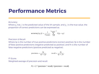
SlideShare a Scribd company logo
MODEL
PERFORMANCEP R E S E N T E D B Y M E G A N V E R B A K E L
Quick refresher
Today we will focus on the simple case of a binary classifier.
A binary classifier is a predictive model where the target can take the value of
0 or 1 (e.g. Predicting whether a customer will reject (0) or accept(1) an offer).
0 and 1 are called classes, where 1 is the positive class (outcome of interest).
We start by taking a historical data set where each row represents one
instance (e.g. a customer) and each column is a feature (e.g. income).
In addition, we need a target column (e.g. an outcome for each customer).
Next, we apply a machine learning algorithm to learn patterns from the
features to predict the probability of each class for each instance (row).
The target values are known for the historical data so we can use it to
understand how the model will perform when applied to new data where
we don't yet know the outcomes.
THEORY
Bias-variance trade-off
Over/under fitting
Finding the performance sweet spot
Data preparation
Performance metrics
Performance plots
PRACTICAL
Walk-through in Python
CONTENT
OUTLINE
Bias Variance Trade-off
Prediction errors can be split into error due to bias and error due to variance
Error due to bias is how far off the predictions are from the true values 
Error due to variance is the variability of model predictions for a given point
As we decrease model bias by increasing complexity, variance increases,
creating a trade-off as we try to minimise both
By thinking of a model with perfect predictions as the bulls-eye, we can
visualise the four scenarios of bias and variance using the below targets:
Low Variance +
Low Bias
Low Variance +
High Bias
High Variance +
High Bias
High Variance +
Low Bias
Over and Under Fitting
Over-fitting occurs when you learn too much detail from the
training data. The model doesn't generalise well, so error increases
when you apply it to new data. 
E.g. if you have one red ice cream in your training data with low
sales, you may incorrectly predict all red ice creams will have low
sales.
Under-fitting is when you don't learn enough detail, so error is high
in both your training and test sets.
Over-fitting increases as you increase complexity (e.g. add more
features, increase depth of trees), resulting in low bias, but high
variance. 
As you decrease complexity, bias increases but variance decreases.
Our job is to find the optimal level of complexity that minimises
error, and balances bias and variance.
Finding the sweet spot 
To find the sweet spot between under/over-fitting test different
levels of model complexity and minimise the total error.
There will always be a trade-off, so you must decide how much of an
increase in variance you will accept for a decrease in bias.
Take into consideration how similar the new data will be to the
training data. 
If very similar, can create a more complex model without worrying
too much about how it will generalise to slightly different data. 
If there is more variation, reduce complexity to improve the stability
of the performance on new data sets.
Must also take into account the importance of 'explainability'. If you
need to be able to explain the model to business stakeholders, a
simpler model may be preferred.
Data: Train/Test Split
To test the performance of a model, split the data into a train set
and a test set. Common splits are 80/20, and 70/30.
Train the model on the training data then apply to the test data to
check if the model works on new (unseen) data (i.e. does it
generalise).
When comparing models, select the model that minimises the
prediction error in the test data.
However, we also want to minimise the performance gap between
the train and test sets (big gap indicates overfitting, low
performance in both indicates under-fitting)
Stratify on the target to ensure the proportion of values in each class
is the same in both the train and test set. This is to maintain the
representation of the original data.
Data: Cross-validation
Cross-validation helps test for over-fitting by checking how the model holds
up when trained and tested on different subsets of the data.
The most common method is k-folds cross validation, where k is the number
of subsets to create (typically between 5 and 10). k-1 subsets are used to train
the model, which is then tested on the set held out. 
At the end, check the mean and standard deviation of the error. If comparing
models, select the model with the lowest mean error and lowest standard
deviation (i.e. minimise bias and variation).
Again, make sure you stratify by your target to ensure the proportion in each
class remains consistent.
https://en.wikipedia.org/wiki/Cross-validation_(statistics)
Performance Plots
Confusion Matrix - A cross tabulation of predicted labels and true labels, used to calculate
recall, precision, and accuracy. Objective in this example: we want to predict which
customers will accept the offer so we can minimise the cost of calling potential customers.
Recall (positive)* = 937 / (937+121) = 0.89 
We correctly predicted 89% of 'accepts'
*Also called True Positive Rate and Sensitivity
Precision (positive) = 937 / (937+212) = 0.82
Of the cases we said would accept, 82% did
Recall (negative)* = 846 / (846+212) = 0.80
* Also called True Negative Rate and Specificity
Precision (negative) = 846 / (846+121) = 0.87
Accuracy = (846+937) / (846+212+121+937) = 0.84
We correctly predicted the label for 84% of cases
Caution: Accuracy is a poor metric if you have class imbalance. If 90% of cases reject, we could be 90% accurate by just
predicting everything will reject. This doesn't help us achieve our objective of understanding which customers will accept. We
therefore have to look at other metrics such as recall and precision for the positive class to understand the prediction error.
True Negative False Positive
False Negative True Positive
Performance Plots
ROC (Receiver Operating Characteristic) - Originally for radio signals, shows the trade-off between
the true positive rate (positive class recall) and the false positive rate (1 - negative class recall) at
different probability thresholds. We want to maximise the TPR to capture as much of the positive
class as possible, while minimising the FPR which is our error or wasted effort.
Area under the curve (AUC) - Measures the area underneath the ROC curve.
0.5 (straight diagonal line) = random (TPR/FPR are equal, the true class is split 50/50)
1 (left corner) = perfect predictions
Performance Plots
Lift & Gain - compares the model to random selection when the data is ordered by the
positive class probability (high to low). For each 10% of the population, the proportion in the
positive class (left graph - lift), and what cumulative proportion have you captured (right
graph - gain)
As hoped, the majority of cases
assigned a high probability for the
positive class were in the positive
class. If we call only the top 10%, over
90% will accept the offer
With the model we can capture > 80% of customers who
will accept the offer while calling only 50% of the total
group, compared to 50% if we called randomly
Performance Metrics
Accuracy:
Where y_hat_i is the predicted value of the ith sample, and y_i is the true value, the
proportion of correct predictions can be expressed as:
Precision & Recall:
Where tp is the number of true positive predictions (correct positive), fp is the number
of false positive predictions (negative predicted as positive), and fn is the number of
false negative predictions (positive predicted as negative).
F1 Score:
Weighted average of precision and recall:
F1 = 2 * (precision * recall) / (precision + recall)
Performance Metrics
ROC_AUC: The area under the ROC curve is the probability a random positive instance
is correctly ranked higher in probability than a random negative instance. The area
under the ROC curve is calculated using the formula for the area of a trapezoid:
Gini co-efficient:
The gini coefficient is ratio of the area between the diagonal line
(perfect equality) and the Lorenz curve (cumulative positive class
proportion) and the total area. B is equal to ROC_AUC - 0.5, thus
the gini co-efficient can be derived from ROC AUC: 
Log Loss (binary):
Where y is the true label, and a probability estimate p=Pr(y=1), the log loss per sample is
the negative log-likelihood of the classifier given the true label:
Gini = A / (A + B)
Gini = (AUC-0.5)*2
https://en.wikipedia.org/wiki/Gini_coefficient
Metrics Summary
Accuracy (0-1) - maximise - of all predictions, the proportion correctly predicted
Recall (0-1) - maximise - of the instances actually in a class, the proportion correctly
predicted as that class (i.e. how many you pick up)
Precision (0-1) - maximise - of the instances predicted to be a class, the proportion
that were correct (i.e. 1-precision is the error or incorrect predictions)
F1 score (0-1) - maximise - weighted average of precision and recall (for binary
classifiers, done for positive class)
ROC_AUC (0-1) - maximise - area under the ROC curve
Gini (0-1) - maximise - a measure of inequality, where a high value indicates a
disproportionate amount of the positive class is represented in the cases with a high
probability (good!)
Log loss (0-1) - minimise - log loss increases as the predicted probability diverges
from the actual label (penalises the model based on how sure it was)
Python Practical
To calculate the performance metrics and create the plots discussed, all you
need is the probabilities for each class, the predicted class (assign a threshold to
the probabilities), and the actual outcomes.
If you are using an sklearn algorithm, these can be easily obtained after you
have fitted the model with the predict and predict_proba methods:
clf = sklearn.ensemble.RandomForestClassifier()
predicted_class = clf.predict(x_test)
probabilities = clf.predict_proba(x_test)
A range of performance metrics are available in the sklearn.metrics module: 
http://scikit-learn.org/stable/modules/classes.html#module-sklearn.metrics

More Related Content

What's hot

Regularization
RegularizationRegularization
Regularization
Darren Yow-Bang Wang
 
Introduction to Machine Learning
Introduction to Machine LearningIntroduction to Machine Learning
Introduction to Machine Learning
Shahar Cohen
 
Artificial Neural Network | Deep Neural Network Explained | Artificial Neural...
Artificial Neural Network | Deep Neural Network Explained | Artificial Neural...Artificial Neural Network | Deep Neural Network Explained | Artificial Neural...
Artificial Neural Network | Deep Neural Network Explained | Artificial Neural...
Simplilearn
 
Chapter - 6 Data Mining Concepts and Techniques 2nd Ed slides Han & Kamber
Chapter - 6 Data Mining Concepts and Techniques 2nd Ed slides Han & KamberChapter - 6 Data Mining Concepts and Techniques 2nd Ed slides Han & Kamber
Chapter - 6 Data Mining Concepts and Techniques 2nd Ed slides Han & Kamber
error007
 
Random Forest and KNN is fun
Random Forest and KNN is funRandom Forest and KNN is fun
Random Forest and KNN is fun
Zhen Li
 
Support Vector Machine ppt presentation
Support Vector Machine ppt presentationSupport Vector Machine ppt presentation
Support Vector Machine ppt presentation
AyanaRukasar
 
DBSCAN : A Clustering Algorithm
DBSCAN : A Clustering AlgorithmDBSCAN : A Clustering Algorithm
DBSCAN : A Clustering Algorithm
Pınar Yahşi
 
SVM Algorithm Explained | Support Vector Machine Tutorial Using R | Edureka
SVM Algorithm Explained | Support Vector Machine Tutorial Using R | EdurekaSVM Algorithm Explained | Support Vector Machine Tutorial Using R | Edureka
SVM Algorithm Explained | Support Vector Machine Tutorial Using R | Edureka
Edureka!
 
2. Data Preprocessing.pdf
2. Data Preprocessing.pdf2. Data Preprocessing.pdf
2. Data Preprocessing.pdf
Jyoti Yadav
 
Machine Learning
Machine LearningMachine Learning
Machine Learning
Shrey Malik
 
Hyperparameter Tuning
Hyperparameter TuningHyperparameter Tuning
Hyperparameter Tuning
Jon Lederman
 
Machine Learning Tutorial Part - 2 | Machine Learning Tutorial For Beginners ...
Machine Learning Tutorial Part - 2 | Machine Learning Tutorial For Beginners ...Machine Learning Tutorial Part - 2 | Machine Learning Tutorial For Beginners ...
Machine Learning Tutorial Part - 2 | Machine Learning Tutorial For Beginners ...
Simplilearn
 
Support Vector Machine and Implementation using Weka
Support Vector Machine and Implementation using WekaSupport Vector Machine and Implementation using Weka
Support Vector Machine and Implementation using Weka
Macha Pujitha
 
Machine learning with ADA Boost
Machine learning with ADA BoostMachine learning with ADA Boost
Machine learning with ADA Boost
Aman Patel
 
Cross validation.pptx
Cross validation.pptxCross validation.pptx
Cross validation.pptx
YouKnowwho28
 
Data Mining: Concepts and Techniques — Chapter 2 —
Data Mining:  Concepts and Techniques — Chapter 2 —Data Mining:  Concepts and Techniques — Chapter 2 —
Data Mining: Concepts and Techniques — Chapter 2 —
Salah Amean
 
Support vector machine
Support vector machineSupport vector machine
Support vector machine
Rishabh Gupta
 
Ensemble Learning and Random Forests
Ensemble Learning and Random ForestsEnsemble Learning and Random Forests
Ensemble Learning and Random Forests
CloudxLab
 
Matrix factorization
Matrix factorizationMatrix factorization
Matrix factorization
Luis Serrano
 
Support Vector Machines- SVM
Support Vector Machines- SVMSupport Vector Machines- SVM
Support Vector Machines- SVM
Carlo Carandang
 

What's hot (20)

Regularization
RegularizationRegularization
Regularization
 
Introduction to Machine Learning
Introduction to Machine LearningIntroduction to Machine Learning
Introduction to Machine Learning
 
Artificial Neural Network | Deep Neural Network Explained | Artificial Neural...
Artificial Neural Network | Deep Neural Network Explained | Artificial Neural...Artificial Neural Network | Deep Neural Network Explained | Artificial Neural...
Artificial Neural Network | Deep Neural Network Explained | Artificial Neural...
 
Chapter - 6 Data Mining Concepts and Techniques 2nd Ed slides Han & Kamber
Chapter - 6 Data Mining Concepts and Techniques 2nd Ed slides Han & KamberChapter - 6 Data Mining Concepts and Techniques 2nd Ed slides Han & Kamber
Chapter - 6 Data Mining Concepts and Techniques 2nd Ed slides Han & Kamber
 
Random Forest and KNN is fun
Random Forest and KNN is funRandom Forest and KNN is fun
Random Forest and KNN is fun
 
Support Vector Machine ppt presentation
Support Vector Machine ppt presentationSupport Vector Machine ppt presentation
Support Vector Machine ppt presentation
 
DBSCAN : A Clustering Algorithm
DBSCAN : A Clustering AlgorithmDBSCAN : A Clustering Algorithm
DBSCAN : A Clustering Algorithm
 
SVM Algorithm Explained | Support Vector Machine Tutorial Using R | Edureka
SVM Algorithm Explained | Support Vector Machine Tutorial Using R | EdurekaSVM Algorithm Explained | Support Vector Machine Tutorial Using R | Edureka
SVM Algorithm Explained | Support Vector Machine Tutorial Using R | Edureka
 
2. Data Preprocessing.pdf
2. Data Preprocessing.pdf2. Data Preprocessing.pdf
2. Data Preprocessing.pdf
 
Machine Learning
Machine LearningMachine Learning
Machine Learning
 
Hyperparameter Tuning
Hyperparameter TuningHyperparameter Tuning
Hyperparameter Tuning
 
Machine Learning Tutorial Part - 2 | Machine Learning Tutorial For Beginners ...
Machine Learning Tutorial Part - 2 | Machine Learning Tutorial For Beginners ...Machine Learning Tutorial Part - 2 | Machine Learning Tutorial For Beginners ...
Machine Learning Tutorial Part - 2 | Machine Learning Tutorial For Beginners ...
 
Support Vector Machine and Implementation using Weka
Support Vector Machine and Implementation using WekaSupport Vector Machine and Implementation using Weka
Support Vector Machine and Implementation using Weka
 
Machine learning with ADA Boost
Machine learning with ADA BoostMachine learning with ADA Boost
Machine learning with ADA Boost
 
Cross validation.pptx
Cross validation.pptxCross validation.pptx
Cross validation.pptx
 
Data Mining: Concepts and Techniques — Chapter 2 —
Data Mining:  Concepts and Techniques — Chapter 2 —Data Mining:  Concepts and Techniques — Chapter 2 —
Data Mining: Concepts and Techniques — Chapter 2 —
 
Support vector machine
Support vector machineSupport vector machine
Support vector machine
 
Ensemble Learning and Random Forests
Ensemble Learning and Random ForestsEnsemble Learning and Random Forests
Ensemble Learning and Random Forests
 
Matrix factorization
Matrix factorizationMatrix factorization
Matrix factorization
 
Support Vector Machines- SVM
Support Vector Machines- SVMSupport Vector Machines- SVM
Support Vector Machines- SVM
 

Similar to Assessing Model Performance - Beginner's Guide

WEKA:Credibility Evaluating Whats Been Learned
WEKA:Credibility Evaluating Whats Been LearnedWEKA:Credibility Evaluating Whats Been Learned
WEKA:Credibility Evaluating Whats Been Learned
weka Content
 
WEKA: Credibility Evaluating Whats Been Learned
WEKA: Credibility Evaluating Whats Been LearnedWEKA: Credibility Evaluating Whats Been Learned
WEKA: Credibility Evaluating Whats Been Learned
DataminingTools Inc
 
Important Classification and Regression Metrics.pptx
Important Classification and Regression Metrics.pptxImportant Classification and Regression Metrics.pptx
Important Classification and Regression Metrics.pptx
Chode Amarnath
 
Machine learning session5(logistic regression)
Machine learning   session5(logistic regression)Machine learning   session5(logistic regression)
Machine learning session5(logistic regression)
Abhimanyu Dwivedi
 
Machine learning session4(linear regression)
Machine learning   session4(linear regression)Machine learning   session4(linear regression)
Machine learning session4(linear regression)
Abhimanyu Dwivedi
 
Logistic regression
Logistic regressionLogistic regression
Logistic regression
Rupak Roy
 
Machine learning algorithms and business use cases
Machine learning algorithms and business use casesMachine learning algorithms and business use cases
Machine learning algorithms and business use cases
Sridhar Ratakonda
 
working with python
working with pythonworking with python
working with python
bhavesh lande
 
Chapter 02-logistic regression
Chapter 02-logistic regressionChapter 02-logistic regression
Chapter 02-logistic regression
Raman Kannan
 
MLlectureMethod.ppt
MLlectureMethod.pptMLlectureMethod.ppt
MLlectureMethod.ppt
butest
 
MLlectureMethod.ppt
MLlectureMethod.pptMLlectureMethod.ppt
MLlectureMethod.ppt
butest
 
Top 100+ Google Data Science Interview Questions.pdf
Top 100+ Google Data Science Interview Questions.pdfTop 100+ Google Data Science Interview Questions.pdf
Top 100+ Google Data Science Interview Questions.pdf
Datacademy.ai
 
Predict Backorder on a supply chain data for an Organization
Predict Backorder on a supply chain data for an OrganizationPredict Backorder on a supply chain data for an Organization
Predict Backorder on a supply chain data for an Organization
Piyush Srivastava
 
MACHINE LEARNING PPT K MEANS CLUSTERING.
MACHINE LEARNING PPT K MEANS CLUSTERING.MACHINE LEARNING PPT K MEANS CLUSTERING.
MACHINE LEARNING PPT K MEANS CLUSTERING.
AmnaArooj13
 
BOOTSTRAPPING TO EVALUATE RESPONSE MODELS: A SAS® MACRO
BOOTSTRAPPING TO EVALUATE RESPONSE MODELS: A SAS® MACROBOOTSTRAPPING TO EVALUATE RESPONSE MODELS: A SAS® MACRO
BOOTSTRAPPING TO EVALUATE RESPONSE MODELS: A SAS® MACRO
Anthony Kilili
 
Advanced Statistics Homework Help
Advanced Statistics Homework HelpAdvanced Statistics Homework Help
Advanced Statistics Homework Help
Excel Homework Help
 
Intro to data science
Intro to data scienceIntro to data science
Intro to data science
ANURAG SINGH
 
Introduction To Data Science Using R
Introduction To Data Science Using RIntroduction To Data Science Using R
Introduction To Data Science Using R
ANURAG SINGH
 
chap4_Parametric_Methods.ppt
chap4_Parametric_Methods.pptchap4_Parametric_Methods.ppt
chap4_Parametric_Methods.ppt
ShayanChowdary
 
Machine learning in credit risk modeling : a James white paper
Machine learning in credit risk modeling : a James white paperMachine learning in credit risk modeling : a James white paper
Machine learning in credit risk modeling : a James white paper
James by CrowdProcess
 

Similar to Assessing Model Performance - Beginner's Guide (20)

WEKA:Credibility Evaluating Whats Been Learned
WEKA:Credibility Evaluating Whats Been LearnedWEKA:Credibility Evaluating Whats Been Learned
WEKA:Credibility Evaluating Whats Been Learned
 
WEKA: Credibility Evaluating Whats Been Learned
WEKA: Credibility Evaluating Whats Been LearnedWEKA: Credibility Evaluating Whats Been Learned
WEKA: Credibility Evaluating Whats Been Learned
 
Important Classification and Regression Metrics.pptx
Important Classification and Regression Metrics.pptxImportant Classification and Regression Metrics.pptx
Important Classification and Regression Metrics.pptx
 
Machine learning session5(logistic regression)
Machine learning   session5(logistic regression)Machine learning   session5(logistic regression)
Machine learning session5(logistic regression)
 
Machine learning session4(linear regression)
Machine learning   session4(linear regression)Machine learning   session4(linear regression)
Machine learning session4(linear regression)
 
Logistic regression
Logistic regressionLogistic regression
Logistic regression
 
Machine learning algorithms and business use cases
Machine learning algorithms and business use casesMachine learning algorithms and business use cases
Machine learning algorithms and business use cases
 
working with python
working with pythonworking with python
working with python
 
Chapter 02-logistic regression
Chapter 02-logistic regressionChapter 02-logistic regression
Chapter 02-logistic regression
 
MLlectureMethod.ppt
MLlectureMethod.pptMLlectureMethod.ppt
MLlectureMethod.ppt
 
MLlectureMethod.ppt
MLlectureMethod.pptMLlectureMethod.ppt
MLlectureMethod.ppt
 
Top 100+ Google Data Science Interview Questions.pdf
Top 100+ Google Data Science Interview Questions.pdfTop 100+ Google Data Science Interview Questions.pdf
Top 100+ Google Data Science Interview Questions.pdf
 
Predict Backorder on a supply chain data for an Organization
Predict Backorder on a supply chain data for an OrganizationPredict Backorder on a supply chain data for an Organization
Predict Backorder on a supply chain data for an Organization
 
MACHINE LEARNING PPT K MEANS CLUSTERING.
MACHINE LEARNING PPT K MEANS CLUSTERING.MACHINE LEARNING PPT K MEANS CLUSTERING.
MACHINE LEARNING PPT K MEANS CLUSTERING.
 
BOOTSTRAPPING TO EVALUATE RESPONSE MODELS: A SAS® MACRO
BOOTSTRAPPING TO EVALUATE RESPONSE MODELS: A SAS® MACROBOOTSTRAPPING TO EVALUATE RESPONSE MODELS: A SAS® MACRO
BOOTSTRAPPING TO EVALUATE RESPONSE MODELS: A SAS® MACRO
 
Advanced Statistics Homework Help
Advanced Statistics Homework HelpAdvanced Statistics Homework Help
Advanced Statistics Homework Help
 
Intro to data science
Intro to data scienceIntro to data science
Intro to data science
 
Introduction To Data Science Using R
Introduction To Data Science Using RIntroduction To Data Science Using R
Introduction To Data Science Using R
 
chap4_Parametric_Methods.ppt
chap4_Parametric_Methods.pptchap4_Parametric_Methods.ppt
chap4_Parametric_Methods.ppt
 
Machine learning in credit risk modeling : a James white paper
Machine learning in credit risk modeling : a James white paperMachine learning in credit risk modeling : a James white paper
Machine learning in credit risk modeling : a James white paper
 

Recently uploaded

The Building Blocks of QuestDB, a Time Series Database
The Building Blocks of QuestDB, a Time Series DatabaseThe Building Blocks of QuestDB, a Time Series Database
The Building Blocks of QuestDB, a Time Series Database
javier ramirez
 
一比一原版(UO毕业证)渥太华大学毕业证如何办理
一比一原版(UO毕业证)渥太华大学毕业证如何办理一比一原版(UO毕业证)渥太华大学毕业证如何办理
一比一原版(UO毕业证)渥太华大学毕业证如何办理
aqzctr7x
 
06-04-2024 - NYC Tech Week - Discussion on Vector Databases, Unstructured Dat...
06-04-2024 - NYC Tech Week - Discussion on Vector Databases, Unstructured Dat...06-04-2024 - NYC Tech Week - Discussion on Vector Databases, Unstructured Dat...
06-04-2024 - NYC Tech Week - Discussion on Vector Databases, Unstructured Dat...
Timothy Spann
 
STATATHON: Unleashing the Power of Statistics in a 48-Hour Knowledge Extravag...
STATATHON: Unleashing the Power of Statistics in a 48-Hour Knowledge Extravag...STATATHON: Unleashing the Power of Statistics in a 48-Hour Knowledge Extravag...
STATATHON: Unleashing the Power of Statistics in a 48-Hour Knowledge Extravag...
sameer shah
 
Palo Alto Cortex XDR presentation .......
Palo Alto Cortex XDR presentation .......Palo Alto Cortex XDR presentation .......
Palo Alto Cortex XDR presentation .......
Sachin Paul
 
一比一原版(CBU毕业证)卡普顿大学毕业证如何办理
一比一原版(CBU毕业证)卡普顿大学毕业证如何办理一比一原版(CBU毕业证)卡普顿大学毕业证如何办理
一比一原版(CBU毕业证)卡普顿大学毕业证如何办理
ahzuo
 
一比一原版(UniSA毕业证书)南澳大学毕业证如何办理
一比一原版(UniSA毕业证书)南澳大学毕业证如何办理一比一原版(UniSA毕业证书)南澳大学毕业证如何办理
一比一原版(UniSA毕业证书)南澳大学毕业证如何办理
slg6lamcq
 
Influence of Marketing Strategy and Market Competition on Business Plan
Influence of Marketing Strategy and Market Competition on Business PlanInfluence of Marketing Strategy and Market Competition on Business Plan
Influence of Marketing Strategy and Market Competition on Business Plan
jerlynmaetalle
 
一比一原版(Bradford毕业证书)布拉德福德大学毕业证如何办理
一比一原版(Bradford毕业证书)布拉德福德大学毕业证如何办理一比一原版(Bradford毕业证书)布拉德福德大学毕业证如何办理
一比一原版(Bradford毕业证书)布拉德福德大学毕业证如何办理
mbawufebxi
 
在线办理(英国UCA毕业证书)创意艺术大学毕业证在读证明一模一样
在线办理(英国UCA毕业证书)创意艺术大学毕业证在读证明一模一样在线办理(英国UCA毕业证书)创意艺术大学毕业证在读证明一模一样
在线办理(英国UCA毕业证书)创意艺术大学毕业证在读证明一模一样
v7oacc3l
 
4th Modern Marketing Reckoner by MMA Global India & Group M: 60+ experts on W...
4th Modern Marketing Reckoner by MMA Global India & Group M: 60+ experts on W...4th Modern Marketing Reckoner by MMA Global India & Group M: 60+ experts on W...
4th Modern Marketing Reckoner by MMA Global India & Group M: 60+ experts on W...
Social Samosa
 
State of Artificial intelligence Report 2023
State of Artificial intelligence Report 2023State of Artificial intelligence Report 2023
State of Artificial intelligence Report 2023
kuntobimo2016
 
Predictably Improve Your B2B Tech Company's Performance by Leveraging Data
Predictably Improve Your B2B Tech Company's Performance by Leveraging DataPredictably Improve Your B2B Tech Company's Performance by Leveraging Data
Predictably Improve Your B2B Tech Company's Performance by Leveraging Data
Kiwi Creative
 
一比一原版(UIUC毕业证)伊利诺伊大学|厄巴纳-香槟分校毕业证如何办理
一比一原版(UIUC毕业证)伊利诺伊大学|厄巴纳-香槟分校毕业证如何办理一比一原版(UIUC毕业证)伊利诺伊大学|厄巴纳-香槟分校毕业证如何办理
一比一原版(UIUC毕业证)伊利诺伊大学|厄巴纳-香槟分校毕业证如何办理
ahzuo
 
Intelligence supported media monitoring in veterinary medicine
Intelligence supported media monitoring in veterinary medicineIntelligence supported media monitoring in veterinary medicine
Intelligence supported media monitoring in veterinary medicine
AndrzejJarynowski
 
原版制作(Deakin毕业证书)迪肯大学毕业证学位证一模一样
原版制作(Deakin毕业证书)迪肯大学毕业证学位证一模一样原版制作(Deakin毕业证书)迪肯大学毕业证学位证一模一样
原版制作(Deakin毕业证书)迪肯大学毕业证学位证一模一样
u86oixdj
 
University of New South Wales degree offer diploma Transcript
University of New South Wales degree offer diploma TranscriptUniversity of New South Wales degree offer diploma Transcript
University of New South Wales degree offer diploma Transcript
soxrziqu
 
Learn SQL from basic queries to Advance queries
Learn SQL from basic queries to Advance queriesLearn SQL from basic queries to Advance queries
Learn SQL from basic queries to Advance queries
manishkhaire30
 
The Ipsos - AI - Monitor 2024 Report.pdf
The  Ipsos - AI - Monitor 2024 Report.pdfThe  Ipsos - AI - Monitor 2024 Report.pdf
The Ipsos - AI - Monitor 2024 Report.pdf
Social Samosa
 
06-04-2024 - NYC Tech Week - Discussion on Vector Databases, Unstructured Dat...
06-04-2024 - NYC Tech Week - Discussion on Vector Databases, Unstructured Dat...06-04-2024 - NYC Tech Week - Discussion on Vector Databases, Unstructured Dat...
06-04-2024 - NYC Tech Week - Discussion on Vector Databases, Unstructured Dat...
Timothy Spann
 

Recently uploaded (20)

The Building Blocks of QuestDB, a Time Series Database
The Building Blocks of QuestDB, a Time Series DatabaseThe Building Blocks of QuestDB, a Time Series Database
The Building Blocks of QuestDB, a Time Series Database
 
一比一原版(UO毕业证)渥太华大学毕业证如何办理
一比一原版(UO毕业证)渥太华大学毕业证如何办理一比一原版(UO毕业证)渥太华大学毕业证如何办理
一比一原版(UO毕业证)渥太华大学毕业证如何办理
 
06-04-2024 - NYC Tech Week - Discussion on Vector Databases, Unstructured Dat...
06-04-2024 - NYC Tech Week - Discussion on Vector Databases, Unstructured Dat...06-04-2024 - NYC Tech Week - Discussion on Vector Databases, Unstructured Dat...
06-04-2024 - NYC Tech Week - Discussion on Vector Databases, Unstructured Dat...
 
STATATHON: Unleashing the Power of Statistics in a 48-Hour Knowledge Extravag...
STATATHON: Unleashing the Power of Statistics in a 48-Hour Knowledge Extravag...STATATHON: Unleashing the Power of Statistics in a 48-Hour Knowledge Extravag...
STATATHON: Unleashing the Power of Statistics in a 48-Hour Knowledge Extravag...
 
Palo Alto Cortex XDR presentation .......
Palo Alto Cortex XDR presentation .......Palo Alto Cortex XDR presentation .......
Palo Alto Cortex XDR presentation .......
 
一比一原版(CBU毕业证)卡普顿大学毕业证如何办理
一比一原版(CBU毕业证)卡普顿大学毕业证如何办理一比一原版(CBU毕业证)卡普顿大学毕业证如何办理
一比一原版(CBU毕业证)卡普顿大学毕业证如何办理
 
一比一原版(UniSA毕业证书)南澳大学毕业证如何办理
一比一原版(UniSA毕业证书)南澳大学毕业证如何办理一比一原版(UniSA毕业证书)南澳大学毕业证如何办理
一比一原版(UniSA毕业证书)南澳大学毕业证如何办理
 
Influence of Marketing Strategy and Market Competition on Business Plan
Influence of Marketing Strategy and Market Competition on Business PlanInfluence of Marketing Strategy and Market Competition on Business Plan
Influence of Marketing Strategy and Market Competition on Business Plan
 
一比一原版(Bradford毕业证书)布拉德福德大学毕业证如何办理
一比一原版(Bradford毕业证书)布拉德福德大学毕业证如何办理一比一原版(Bradford毕业证书)布拉德福德大学毕业证如何办理
一比一原版(Bradford毕业证书)布拉德福德大学毕业证如何办理
 
在线办理(英国UCA毕业证书)创意艺术大学毕业证在读证明一模一样
在线办理(英国UCA毕业证书)创意艺术大学毕业证在读证明一模一样在线办理(英国UCA毕业证书)创意艺术大学毕业证在读证明一模一样
在线办理(英国UCA毕业证书)创意艺术大学毕业证在读证明一模一样
 
4th Modern Marketing Reckoner by MMA Global India & Group M: 60+ experts on W...
4th Modern Marketing Reckoner by MMA Global India & Group M: 60+ experts on W...4th Modern Marketing Reckoner by MMA Global India & Group M: 60+ experts on W...
4th Modern Marketing Reckoner by MMA Global India & Group M: 60+ experts on W...
 
State of Artificial intelligence Report 2023
State of Artificial intelligence Report 2023State of Artificial intelligence Report 2023
State of Artificial intelligence Report 2023
 
Predictably Improve Your B2B Tech Company's Performance by Leveraging Data
Predictably Improve Your B2B Tech Company's Performance by Leveraging DataPredictably Improve Your B2B Tech Company's Performance by Leveraging Data
Predictably Improve Your B2B Tech Company's Performance by Leveraging Data
 
一比一原版(UIUC毕业证)伊利诺伊大学|厄巴纳-香槟分校毕业证如何办理
一比一原版(UIUC毕业证)伊利诺伊大学|厄巴纳-香槟分校毕业证如何办理一比一原版(UIUC毕业证)伊利诺伊大学|厄巴纳-香槟分校毕业证如何办理
一比一原版(UIUC毕业证)伊利诺伊大学|厄巴纳-香槟分校毕业证如何办理
 
Intelligence supported media monitoring in veterinary medicine
Intelligence supported media monitoring in veterinary medicineIntelligence supported media monitoring in veterinary medicine
Intelligence supported media monitoring in veterinary medicine
 
原版制作(Deakin毕业证书)迪肯大学毕业证学位证一模一样
原版制作(Deakin毕业证书)迪肯大学毕业证学位证一模一样原版制作(Deakin毕业证书)迪肯大学毕业证学位证一模一样
原版制作(Deakin毕业证书)迪肯大学毕业证学位证一模一样
 
University of New South Wales degree offer diploma Transcript
University of New South Wales degree offer diploma TranscriptUniversity of New South Wales degree offer diploma Transcript
University of New South Wales degree offer diploma Transcript
 
Learn SQL from basic queries to Advance queries
Learn SQL from basic queries to Advance queriesLearn SQL from basic queries to Advance queries
Learn SQL from basic queries to Advance queries
 
The Ipsos - AI - Monitor 2024 Report.pdf
The  Ipsos - AI - Monitor 2024 Report.pdfThe  Ipsos - AI - Monitor 2024 Report.pdf
The Ipsos - AI - Monitor 2024 Report.pdf
 
06-04-2024 - NYC Tech Week - Discussion on Vector Databases, Unstructured Dat...
06-04-2024 - NYC Tech Week - Discussion on Vector Databases, Unstructured Dat...06-04-2024 - NYC Tech Week - Discussion on Vector Databases, Unstructured Dat...
06-04-2024 - NYC Tech Week - Discussion on Vector Databases, Unstructured Dat...
 

Assessing Model Performance - Beginner's Guide

  • 1. MODEL PERFORMANCEP R E S E N T E D B Y M E G A N V E R B A K E L
  • 2. Quick refresher Today we will focus on the simple case of a binary classifier. A binary classifier is a predictive model where the target can take the value of 0 or 1 (e.g. Predicting whether a customer will reject (0) or accept(1) an offer). 0 and 1 are called classes, where 1 is the positive class (outcome of interest). We start by taking a historical data set where each row represents one instance (e.g. a customer) and each column is a feature (e.g. income). In addition, we need a target column (e.g. an outcome for each customer). Next, we apply a machine learning algorithm to learn patterns from the features to predict the probability of each class for each instance (row). The target values are known for the historical data so we can use it to understand how the model will perform when applied to new data where we don't yet know the outcomes.
  • 3. THEORY Bias-variance trade-off Over/under fitting Finding the performance sweet spot Data preparation Performance metrics Performance plots PRACTICAL Walk-through in Python CONTENT OUTLINE
  • 4. Bias Variance Trade-off Prediction errors can be split into error due to bias and error due to variance Error due to bias is how far off the predictions are from the true values  Error due to variance is the variability of model predictions for a given point As we decrease model bias by increasing complexity, variance increases, creating a trade-off as we try to minimise both By thinking of a model with perfect predictions as the bulls-eye, we can visualise the four scenarios of bias and variance using the below targets: Low Variance + Low Bias Low Variance + High Bias High Variance + High Bias High Variance + Low Bias
  • 5. Over and Under Fitting Over-fitting occurs when you learn too much detail from the training data. The model doesn't generalise well, so error increases when you apply it to new data.  E.g. if you have one red ice cream in your training data with low sales, you may incorrectly predict all red ice creams will have low sales. Under-fitting is when you don't learn enough detail, so error is high in both your training and test sets. Over-fitting increases as you increase complexity (e.g. add more features, increase depth of trees), resulting in low bias, but high variance.  As you decrease complexity, bias increases but variance decreases. Our job is to find the optimal level of complexity that minimises error, and balances bias and variance.
  • 6. Finding the sweet spot  To find the sweet spot between under/over-fitting test different levels of model complexity and minimise the total error. There will always be a trade-off, so you must decide how much of an increase in variance you will accept for a decrease in bias. Take into consideration how similar the new data will be to the training data.  If very similar, can create a more complex model without worrying too much about how it will generalise to slightly different data.  If there is more variation, reduce complexity to improve the stability of the performance on new data sets. Must also take into account the importance of 'explainability'. If you need to be able to explain the model to business stakeholders, a simpler model may be preferred.
  • 7. Data: Train/Test Split To test the performance of a model, split the data into a train set and a test set. Common splits are 80/20, and 70/30. Train the model on the training data then apply to the test data to check if the model works on new (unseen) data (i.e. does it generalise). When comparing models, select the model that minimises the prediction error in the test data. However, we also want to minimise the performance gap between the train and test sets (big gap indicates overfitting, low performance in both indicates under-fitting) Stratify on the target to ensure the proportion of values in each class is the same in both the train and test set. This is to maintain the representation of the original data.
  • 8. Data: Cross-validation Cross-validation helps test for over-fitting by checking how the model holds up when trained and tested on different subsets of the data. The most common method is k-folds cross validation, where k is the number of subsets to create (typically between 5 and 10). k-1 subsets are used to train the model, which is then tested on the set held out.  At the end, check the mean and standard deviation of the error. If comparing models, select the model with the lowest mean error and lowest standard deviation (i.e. minimise bias and variation). Again, make sure you stratify by your target to ensure the proportion in each class remains consistent. https://en.wikipedia.org/wiki/Cross-validation_(statistics)
  • 9. Performance Plots Confusion Matrix - A cross tabulation of predicted labels and true labels, used to calculate recall, precision, and accuracy. Objective in this example: we want to predict which customers will accept the offer so we can minimise the cost of calling potential customers. Recall (positive)* = 937 / (937+121) = 0.89  We correctly predicted 89% of 'accepts' *Also called True Positive Rate and Sensitivity Precision (positive) = 937 / (937+212) = 0.82 Of the cases we said would accept, 82% did Recall (negative)* = 846 / (846+212) = 0.80 * Also called True Negative Rate and Specificity Precision (negative) = 846 / (846+121) = 0.87 Accuracy = (846+937) / (846+212+121+937) = 0.84 We correctly predicted the label for 84% of cases Caution: Accuracy is a poor metric if you have class imbalance. If 90% of cases reject, we could be 90% accurate by just predicting everything will reject. This doesn't help us achieve our objective of understanding which customers will accept. We therefore have to look at other metrics such as recall and precision for the positive class to understand the prediction error. True Negative False Positive False Negative True Positive
  • 10. Performance Plots ROC (Receiver Operating Characteristic) - Originally for radio signals, shows the trade-off between the true positive rate (positive class recall) and the false positive rate (1 - negative class recall) at different probability thresholds. We want to maximise the TPR to capture as much of the positive class as possible, while minimising the FPR which is our error or wasted effort. Area under the curve (AUC) - Measures the area underneath the ROC curve. 0.5 (straight diagonal line) = random (TPR/FPR are equal, the true class is split 50/50) 1 (left corner) = perfect predictions
  • 11. Performance Plots Lift & Gain - compares the model to random selection when the data is ordered by the positive class probability (high to low). For each 10% of the population, the proportion in the positive class (left graph - lift), and what cumulative proportion have you captured (right graph - gain) As hoped, the majority of cases assigned a high probability for the positive class were in the positive class. If we call only the top 10%, over 90% will accept the offer With the model we can capture > 80% of customers who will accept the offer while calling only 50% of the total group, compared to 50% if we called randomly
  • 12. Performance Metrics Accuracy: Where y_hat_i is the predicted value of the ith sample, and y_i is the true value, the proportion of correct predictions can be expressed as: Precision & Recall: Where tp is the number of true positive predictions (correct positive), fp is the number of false positive predictions (negative predicted as positive), and fn is the number of false negative predictions (positive predicted as negative). F1 Score: Weighted average of precision and recall: F1 = 2 * (precision * recall) / (precision + recall)
  • 13. Performance Metrics ROC_AUC: The area under the ROC curve is the probability a random positive instance is correctly ranked higher in probability than a random negative instance. The area under the ROC curve is calculated using the formula for the area of a trapezoid: Gini co-efficient: The gini coefficient is ratio of the area between the diagonal line (perfect equality) and the Lorenz curve (cumulative positive class proportion) and the total area. B is equal to ROC_AUC - 0.5, thus the gini co-efficient can be derived from ROC AUC:  Log Loss (binary): Where y is the true label, and a probability estimate p=Pr(y=1), the log loss per sample is the negative log-likelihood of the classifier given the true label: Gini = A / (A + B) Gini = (AUC-0.5)*2 https://en.wikipedia.org/wiki/Gini_coefficient
  • 14. Metrics Summary Accuracy (0-1) - maximise - of all predictions, the proportion correctly predicted Recall (0-1) - maximise - of the instances actually in a class, the proportion correctly predicted as that class (i.e. how many you pick up) Precision (0-1) - maximise - of the instances predicted to be a class, the proportion that were correct (i.e. 1-precision is the error or incorrect predictions) F1 score (0-1) - maximise - weighted average of precision and recall (for binary classifiers, done for positive class) ROC_AUC (0-1) - maximise - area under the ROC curve Gini (0-1) - maximise - a measure of inequality, where a high value indicates a disproportionate amount of the positive class is represented in the cases with a high probability (good!) Log loss (0-1) - minimise - log loss increases as the predicted probability diverges from the actual label (penalises the model based on how sure it was)
  • 15. Python Practical To calculate the performance metrics and create the plots discussed, all you need is the probabilities for each class, the predicted class (assign a threshold to the probabilities), and the actual outcomes. If you are using an sklearn algorithm, these can be easily obtained after you have fitted the model with the predict and predict_proba methods: clf = sklearn.ensemble.RandomForestClassifier() predicted_class = clf.predict(x_test) probabilities = clf.predict_proba(x_test) A range of performance metrics are available in the sklearn.metrics module:  http://scikit-learn.org/stable/modules/classes.html#module-sklearn.metrics